Exact Solution of the Multi-trip Inventory Routing Problem using a
Pseudo-polynomial Model
Nuno Braga
1
, Cl
´
audio Alves
1
and Rita Macedo
2
1
Universidade do Minho, 4710-057, Braga, Portugal
2
Institut de Recherche Technologique Railenium, F-59300, Famars, France
Keywords:
Inventory Routing Problem, Integer Linear Programing, Network Flow Models, Multi-trip.
Abstract:
In this paper, we address an inventory routing problem where a vehicle can perform more than one trip in
a working day. This problem was denominated multi-trip vehicle routing problem. In this problem a set of
customers with demand for the planning horizon must be satisfied by a supplier. The supplier, with a set of
vehicles, delivers the demand using pre-calculated valid routes that define the schedule of the delivery of goods
on the planning horizon. The problem is solved with a pseudo-polynomial network flow model that is solved
exactly in a set of instances adapted from the literature. An extensive set of computational experiments on
these instances were conducted varying a set of parameters of the model. The results obtained with this model
show that it is possible to solve instances up to 50 customers and with 15 periods in a reasonable computational
time.
1 INTRODUCTION
The vehicle routing problem can be applied in real
cases on logistics companies in order to reduce trans-
portation costs, which include, among others, costs
associated with drivers, vehicles or fuel. The integra-
tion of this problem with the inventory management
can reflect in considerable savings, since this provides
a more efficient management of the resources than
the one achieved through the local optimization of the
two problems separately.
In the inventory routing problem the goal is to
minimize the total transportation cost from the sup-
plier to the customer, so that the customer maintains
an inventory level that will satisfy the demand in each
period of a given planning horizon, reducing also pos-
sible storage costs.
This problem can incorporate a time horizon infor-
mation, inventory management policies, routes, fleet
type and size (Coelho et al., 2014). Routes are con-
sidered to be direct or not, whether a single customer
or more are visited, respectively (Coelho et al., 2014).
The planning horizon is considered finite if it is de-
fined for a short period, or infinite when the sched-
ule of routes is carried out for a long period of time
(Coelho et al., 2014; Bertazzi and Speranza, 2013).
Typically, the goal is to minimize the overall trans-
portation costs, reducing penalties associated with in-
ventory level, which typically represent storage costs
(Bertazzi and Speranza, 2013).
Several practical applications have been imple-
mented in industry, which enable companies to re-
duce inventory and transportation costs improving the
quality of service. A recent study describes the im-
plementation of this problem in a fuel distribution
company (Hanczar, 2012). Another study describes
an application of the problem in a company with a
fleet of ships that delivers chemicals to warehouses
located throughout the world (Miller, 1987). The
authors describe an integer programming model that
was successfully implemented in this company. The
inventary routing problem was also considered in the
daily strategy of a company that provides calcium car-
bonate throughout Europe and it allowed to achieve
a reduction in millions of dollars of costs per year
(Dauz
`
ere-P
´
er
`
es et al., 2007). In addition, different
approaches of this problem have also been applied
in the maritime industry (Al-Khayyal and Hwang,
2007; Song and Furman, 2013; Persson and G
¨
othe-
Lundgren, 2005; Grnhaug et al., 2010).
The problem explored in this paper is the inven-
tory routing problem that allowed the vehicles to carry
out more than one route in each period of the planning
horizon and therefore it was denominated multi-trip
inventory routing problem. The consideration of mul-
tiple routes can provide advantages, in the sense that
250
Braga N., Alves C. and Macedo R.
Exact Solution of the Multi-trip Inventory Routing Problem using a Pseudo-polynomial Model.
DOI: 10.5220/0006118502500257
In Proceedings of the 6th International Conference on Operations Research and Enterprise Systems (ICORES 2017), pages 250-257
ISBN: 978-989-758-218-9
Copyright
c
 2017 by SCITEPRESS – Science and Technology Publications, Lda. All rights reserved

the cost of the vehicle is usually fixed for a period
of the planning horizon, therefore reducing the costs
at this level. On the other hand, the consideration of
this variant with multiple routes makes the problem,
which is already difficult to solve, even more difficult.
Since there is an increasing interest in applying
this problem in practical cases in industry, several
heuristics and exact algorithms have been proposed
by several authors in the literature. The difficulty
of solving the inventory routing problems has been
mostly motivated by the development of heuristics,
which in many cases show good results (Herer and
Levy, 1997; Archetti et al., 2011; Cordeau et al.,
2015; Hemmati et al., 2015). In a recent paper, the
inventory routing problem with multiple products and
vehicles was solved with an exact model (Coelho and
Laporte, 2013). The authors describe an integer pro-
gramming model, to which are also added valid in-
equalities with the objective of strengthening it. In
the model a branch-and-cut is proposed that is able to
solve instances with a maximum of 5 vehicles, 5 prod-
ucts, 7 periods and 50 customers. In another prob-
lem with a constant customers demand the authors re-
sorted to a Lagrangian relaxation method that derives
lower and upper bounds for the model in order to ob-
tain good quality solutions in acceptable times (Zhong
and Aghezzaf, 2012). In another paper it is also pro-
posed a method of Lagrangian relaxation combined
with a subgradient method, able to solve instances up
to 200 customers (Yu et al., 2008). Two integer pro-
gramming models were proposed to solve the inven-
tory routing problem when the inventory is managed
by the supplier and when it is managed by the cus-
tomer, comparing the two approaches (Archetti and
Speranza, 2016).
The multi-trip inventory routing problem is typi-
cally more difficult to resolve as compared with the
usual vehicle routing problem. This variant was re-
viewed elsewhere (S¸en and Blbl, 2008). Since this is
not a trivial problem, several heuristic methods have
been proposed. A tabu search algorithm is also de-
scribed to solve this problem (Taillard et al., 1996).
The same problem was addressed with a heuristic al-
gorithm also using tabu search (Brando and Mercer,
1998). The use of constructive heuristic with three
phases was also proposed (Petch and Salhi, 2003). An
adaptive memory procedure was described (Olivera
and Viera, 2007), and the results were compared with
those obtained with others from the literature (Tail-
lard et al., 1996; Brando and Mercer, 1998; Petch and
Salhi, 2003). A genetic algorithm was also proposed,
for the first time, to solve this problem (Salhi and
Petch, 2007). A vehicle routing problem with multi-
ple routes and additional accessibility constraints was
studied using a tabu search algorithm that involved in-
stances up to 1000 customers (Alonso et al., 2008).
An exact integer programming method was pro-
posed for the problem of routing with a single vehi-
cle with time windows and multiple routes (Azi et al.,
2007). The algorithm is divided in two phases: first,
all valid routes are generated and in the second phase
routes are affected at different periods of the plan-
ning horizon. The authors further generalize the al-
gorithm for the case of multiple vehicles (Azi et al.,
2010). The authors resorted to a column generation
algorithm able to solve instances with a number of
customers between 25 and 50.
A pseudo-polynomial network flow model was
used to solve the vehicle routing problem with time
windows and multiple routes (Macedo et al., 2011).
In the model, the underlying graph vertices corre-
spond to instants of time of the planning horizon, and
the arcs define valid routes. It is proposed an exact al-
gorithm that considers an iterative disaggregation of
the vertices of the graph, which are first aggregated
to obtain a smaller model, and thus easier to solve.
The model proposed in this article is similar to the
one here described (Macedo et al., 2011) in the sense
that it uses a pseudo-polynomial network flow model,
the arcs define valid routes and the vertices also cor-
respond to instances of time.
In section 2 we present the definition of the prob-
lem, showing also an example. On section 3 it is for-
mally presented the pseudo-polynomial network flow
model to solve this problem. In section 4 the com-
putational results are shown and finally, some conclu-
sions are presented in section 5.
2 MULTI-TRIP INVENTORY
ROUTING PROBLEM
2.1 Definition
The class of inventory routing problems considers a
context in which one or more types of products are
shipped from a supplier to a set of customers through
a fleet of vehicles.
In this problem the customers demand should be
satisfied during several periods of a planning horizon.
What differentiates this class of problems, from the
vehicle routing problem is the fact that the supplier
manages the inventory of the customer, i.e., the prod-
uct amount supplied to each customer in each period
is not necessarily equal to their demands. The prod-
ucts deliveries must be carried out in such a way that
the customers have available at each period, the re-
Exact Solution of the Multi-trip Inventory Routing Problem using a Pseudo-polynomial Model
251

quired amount of product.
In this paper, a variant of this problem is addressed
that considers the vehicle routing problem with mul-
tiple routes, which means that each vehicle can be al-
located to more than one route in each period of the
planning horizon.
We consider that a fleet of vehicles is located in a
warehouse, which supplies a set of customers with a
single type of product.
The objective of this problem is to determine the
optimal set of routes that minimize the total trans-
portation cost, and any storage costs in the customer.
That is, whenever an order is delivered before the set
period, incurs in a penalty proportional to the costs
of storage of products in the customer. On the other
hand, it is considered that customers have an unlim-
ited storage capacity. With regard to anticipated de-
liveries, they can not be phased. This means that all
demand for a period is delivered in a single visit to the
corresponding customer, whether made on the same
period or in previous periods.
In this problem, the number of available vehicles
is limited, as well as the capacity of each vehicle, and
the load in each route can not exceed its capacity. It
is assumed that each unit of the product transported
occupies a unit of volume on the vehicle and the time
spent on transportation is equivalent to the distance
traveled. Each vehicle can carry out various routes
per period, so that, the sum of their lengths does not
exceed the duration of a working day.
2.2 Data and Parameters
To clarify the formal presentation of the problem, we
provide below an exhaustive list of parameters that
characterise it:
− D = {0}: warehouse;
− S = {1, . . . , N}: customers;
− T = {1, . . . , τ}: time periods of the planning hori-
zon.
The warehouse is associated with the index 0.
Customers are located within a certain distance from
the warehouse, distributed according to their cartesian
coordinates. The planning horizon defines the time
period for which deliveries to customers will have to
be made. This period will subsequently be divided
into units of time referred to as work day.
We consider that a customer cannot be visited
more than once in each time period and there is a
single type of product. Furthermore, we assume that
a visit to a customer at a time t requires the deliv-
ery of the demand for that period, and eventually the
later periods. Stock-outs are not allowed, i.e., all cus-
tomers must imperatively have at their disposal, in
each period, the required quantities of products. Fi-
nally, it is considered that there is no initial stock in
customers, i.e., at time period 0 of the planning hori-
zon the customers do not have at their disposal any
stock.
Below we present the problem data:
− C: vehicle capacity (homogeneous fleet);
− F: number of available vehicles;
− W : duration of a working day;
− d
t
i
: demand of customer i on time period t;
− N
max
: maximum number of customers visited by
route.
Some additional settings:
− Ψ
t
: set of valid routes in the period t;
− N
r
: set of customers visited by route r;
− α
t
0
irt
: equal to 1 if the route r delivers the demand
of the customers i in the period t, or equal to 0
otherwise;
− a route r is characterised by a set of customers
(visited by the route) and the periods of demands
that are delivered as part of the same route.
The costs considered in this problem are:
− C
v
: fixed cost for using a vehicle in a working day;
− C
r
: transportation cost associated with the route r;
− C
h
i
: storage cost of a unit of product on the cus-
tomers i for a period of time;
− C
H
t
r
: total cost of storage associated with the route
r (C
H
t
r
=
∑
i∈N
r
C
h
i
t
i
r
, being t
i
r
the total waiting time
until the product is consumed on the customer i
delivered through the route r).
2.3 Example of a Problem Instance
Example 1. Consider the example of an instance for
the inventory routing problem.
The Table 1 indicates all the parameters that de-
fine it. Table 1a defines the location of the warehouse,
and Table 1b defines the capacity of the vehicles (C),
the fleet size (F), the duration of a working day (W ),
the number os periods of the planning horizon (τ) and
the number of customers (N). In Table 1c are repre-
sented the customer cartesian coordinates (x, y), as
well as the storage costs for each customer (C
h
i
). Fi-
nally, Table 1d defines the demands d
t
i
in the period t
for the customer i.
The graphical representation of this instance can
be observed in Figure 1, showing the warehouse and
ICORES 2017 - 6th International Conference on Operations Research and Enterprise Systems
252

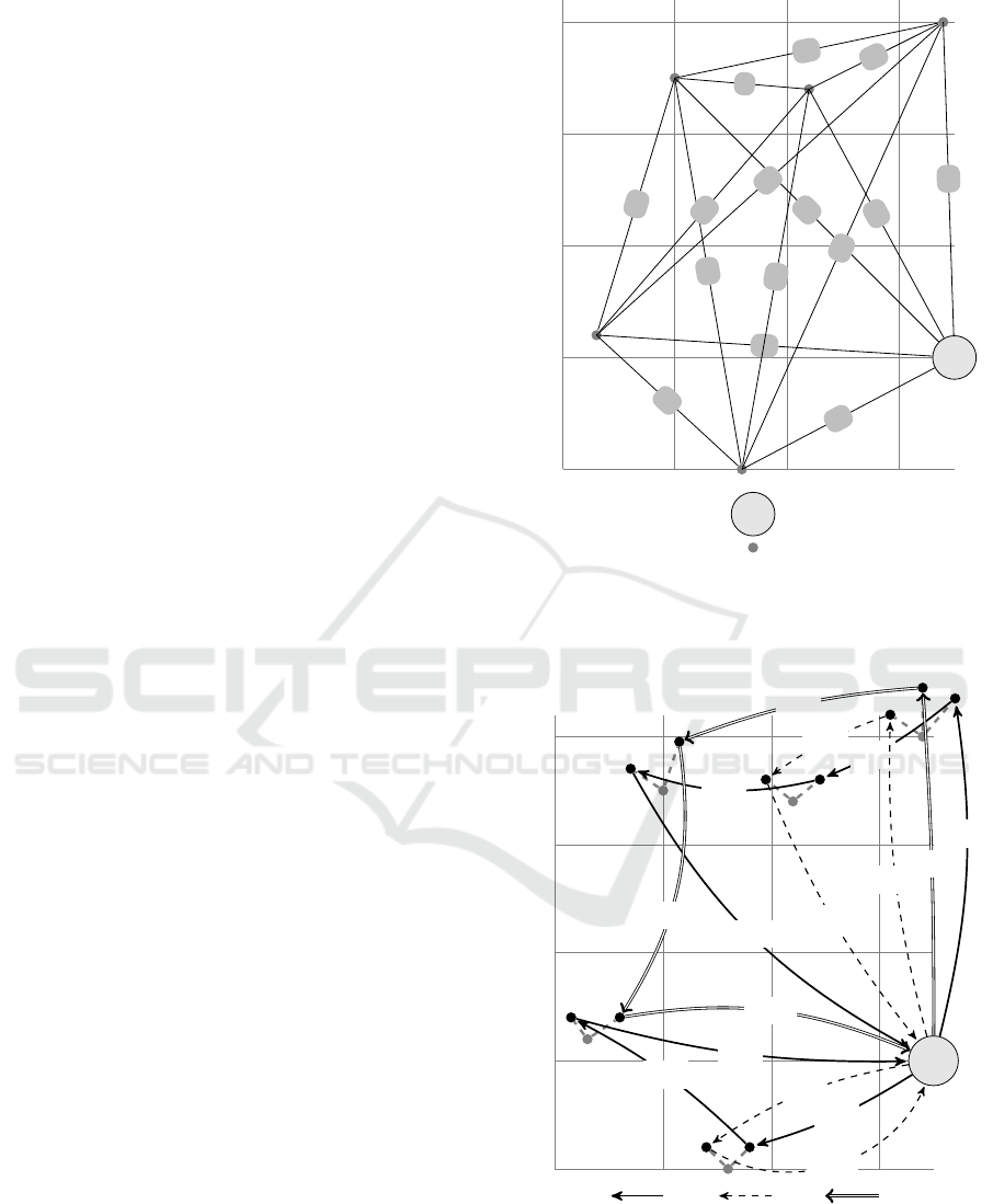
Table 1: Example of an instance of the inventory routing
problem. (a) Warehouse location data, (b) general data of
the problem, (c) customer data and (d) customer demands.
A 10 20
(a)
C 10
C
v
20
F 5
W 120
T 3
N 5
(b)
x y C
h
i
9 50 24
-9 10 15
-22 22 3
-15 45 9
-3 44 12
(c)
t i d
t
i
1 1 4
1 2 2
1 3 2
1 4 2
1 5 2
2 1 2
2 2 2
2 3 2
2 4 2
2 5 2
3 1 4
3 2 2
3 3 2
3 4 2
3 5 3
(d)
the customers distributed according to their cartesian
coordinates. All connections between customers and
warehouse (supplier) are also represented, as well
as the corresponding distances to be traveled in this
route.
Figure 2 represents a valid solution for this in-
stance, which has in the first period a cost of 214,
in the second 198 and in the third and last 131, with
a total cost of 543. In this case, it is not possible to
use a single vehicle in the first period, since the dis-
tance that the vehicle would have to travel to deliver
all customer demands is greater than 120 (length of a
work day). Thus, two vehicles are scheduled for the
routes for the first period, and in each of the routes it
is delivered the demand for further periods, in partic-
ular customers 3 and 4. These deliveries in later peri-
ods incur in a penalty for each unit in storage. In the
second period, it may resort to a single vehicle that
performs two routes. In the third period, a single ve-
hicle performs the remaining deliveries to customers
where the demands have not yet been satisfied, mak-
ing use of a single route. In this latter period there is
no storage costs since all demands are satisfied and
consumed in this period. In this figure, the informa-
tion relative to the demand is denoted by d
t
i
, and can
exist for later periods. The information about the dis-
tance (l) traveled and the volume (v) occupied on the
vehicle in the route is defined in the arcs as [l|v]. Ta-
ble 2 discriminates the objective function values for
the three periods shown in Figure 1.
−25 −15 −5 5
10
20
30
40
50
Wharehouse
Customers
i = 1
i = 2
i = 3
i = 4
i = 5
30
21
32
35
27
44
42
25
13
18
36
35
24
29
4
Figure 1: Instance graphical representation with a ware-
house, customers and their distances located in midway of
the connections.
−25 −15 −5 5
10
20
30
40
50
[d
3
1
]
[d
2
1
]
[d
1
1
]
[d
2
2
, d
3
2
]
[d
1
2
]
[d
1
3
, d
2
3
]
[d
3
3
]
[d
1
4
, d
2
4
]
[d
3
4
]
[d
2
5
, d
3
5
]
[d
1
5
]
[30|10]
[43|6]
[47|4]
[82|0]
[21|6]
[39|4]
[71|0]
[30|7]
[43|5]
[70|0]
[91|4]
[112|0]
[30|8]
[55|4]
[79|2]
[111|0]
Period 1
Period 2
Period 3
Figure 2: Valid solution to the inventory routing problem
instance of Example 1. In the middle of the connection
between each customers is shown the distance traveled, as
well as the volume of the goods on the vehicle in the route.
Exact Solution of the Multi-trip Inventory Routing Problem using a Pseudo-polynomial Model
253

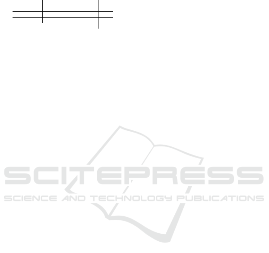
Table 2: Objective function values for the three periods.
T C
r
C
v
C
h
i
total
1 82 + 71 20 + 20 9 × 2 + 3 × 2 214
2 112 20 12 × 3 + 15 × 2 198
3 111 20 0 131
543
3 A NETWORK FLOW MODEL
FOR THE MULTI-TRIP
INVENTORY ROUTING
PROBLEM
In this section, we describe a new integer program-
ming model for the multi-trip inventory routing prob-
lem.
This network flow model is defined in a set of
acyclic and direct graphs, one for each period of the
planning horizon, denoted by G
t
= (V, A
t
), t ∈ T and
V is a set of vertices V = {0, . . . , W + 1}, and A
t
is
the set of arcs that represent the set of all valid routes
in the period t ∈ T , as well as the waiting time in the
warehouse. A flow that runs through the graph repre-
sents a working day of a vehicle, i.e., the sequence of
routes and waiting times this performs from the mo-
ment 0 until time instant w of a given planning hori-
zon. A route is defined by a sequence of customers
to visit, as well as the respective product amounts to
deliver to each customer. In order for a route to be
valid, the sum of the quantities of products to be de-
livered to each customer must not exceed the capacity
of the vehicle, and the necessary travel time cannot
exceed a working day (a period of the planning hori-
zon). Note that the same route can start at different
instants, keeping it valid. The set of all valid routes is
generated in advance, and the variable x
t
uvr
represents
the route r that starts at the instant u and ends at time
v of period t ∈ T . Routes are generated through a re-
cursive process that will exclude routes violating the
vehicle capacity (C) and/or a maximum duration (W )
of the route.
min
∑
t∈T
∑
(u,v)
r
∈Ψ
t
C
r
x
t
uvr
+C
v
∑
t∈T
∑
(0,v)
r
∈Ψ
t
x
t
0vr
+
∑
t∈T
∑
(u,v)
r
∈Ψ
t
C
H
t
r
x
t
uvr
(1)
s.t.
∑
t∈T,t≤t
0
∑
(u,v)
r
∈Ψ
t
|i∈N
r
α
t
0
irt
x
t
uvr
= 1, ∀i ∈ S, t
0
∈ T, (2)
∑
(0,v)
r
∈Ψ
t
x
t
0vr
≤ F, ∀t ∈ T, (3)
−
∑
(u,v)
r
∈Ψ
t
x
t
uvr
+
∑
(v,y)
s
∈Ψ
t
x
t
vys
=



0, if v = 1, . . . , W − 1,
−
∑
(0,v)
r
∈Ψ
t
x
t
0vr
, if v = W,
∀t ∈ T, (4)
x
t
uvr
∈ {0, 1}, ∀(u, v)
r
∈ Ψ
t
, ∀t ∈ T. (5)
The objective function (1) represents the sum of
the transportation costs of the traveled routes C
r
, the
cost of the vehicles used C
v
, and daily storage costs
per item C
H
i
.
Restrictions (2) ensure that deliveries of demands
of all periods, for each of the customers are met by
one and only one of the traveled routes. This deliv-
ery can take place on the same period or in previous
periods.
Restrictions (3) impose that more than F vehicles
in each period t are not used. Conservation flow is
ensured by the restrictions (4).
Example 2. The graph from Figure 3 represents a
valid solution from Figure 2 of Example 1.
These graphs have a dimension W = 120 which
represents the duration of a working day, being 0 the
beginning and W the end. The set of arcs corresponds
to the represented traveled routes. Each vertice de-
fines a time instant and each arch represents a route
traveled to visit a series of customers. These flows
are the arcs defined for the three periods, in the first
one two vehicles perform a route each, in the second
period a single vehicle performs two routes and in
the third and final period a vehicle performs a single
route. This is a valid solution for instance Example 1.
4 COMPUTATIONAL RESULTS
To evaluate the performance of the model, it was used
a set of instances adapted from the literature (Moin
et al., 2010).
A set of 32 instances was generated, and in all
the duration of the planning horizon the working day
is W = 140. There are two instances for each com-
bination of parameters: number of customers N ∈
{10, 20, 40, 50} and number of periods of the plan-
ning horizon τ ∈ {3, 5, 10, 15}.
With this set of instances, different tests were per-
formed varying the capacity of the vehicles. It is con-
sidered C ∈ {10, 13, 20}, so that, for all instances all
the demands are higher than 20%, 15% and 10% of
vehicle capacity, respectively. It was also considered
an additional constraint on the maximum number of
ICORES 2017 - 6th International Conference on Operations Research and Enterprise Systems
254

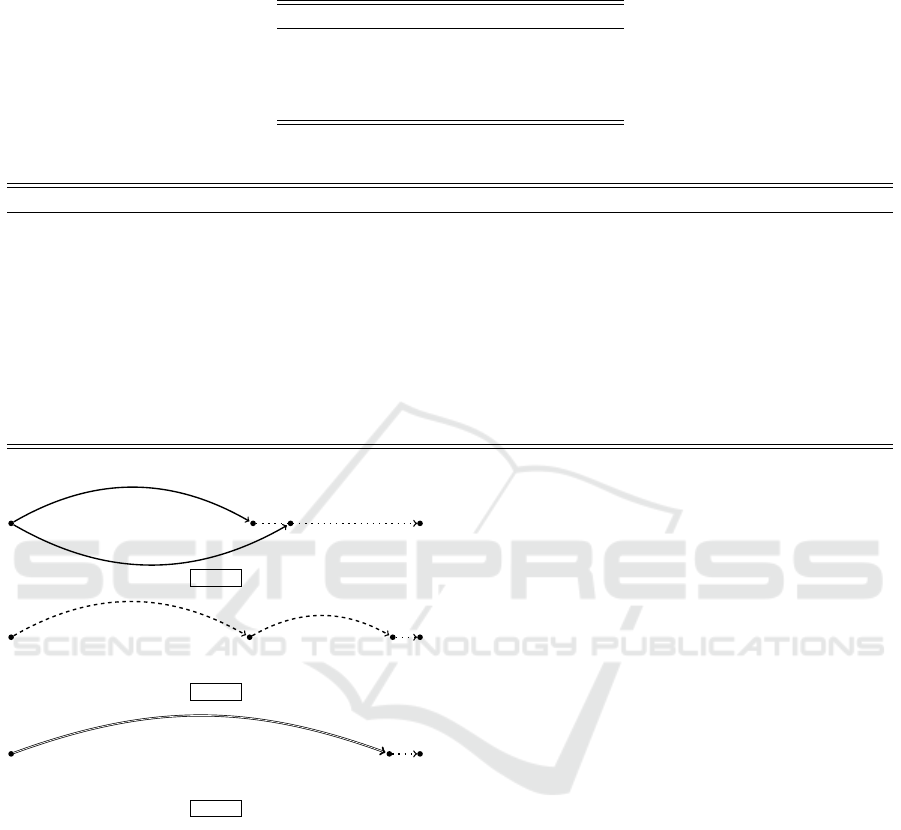
Table 3: Summary of instances solved to optimality / instances in which the model found a solution / number of instances to
solve.
N
max
C = 10 C = 13 C = 20
3 12/32/50 12/30/50 12/20/40
4 12/22/50 8/20/20 8/12/20
5 12/18/40 11/12/20 -
10 12/18/40 10/12/20 -
Table 4: Average values of instances solved with different parameters.
C N
max
¯
t
r
¯
t
m
¯
t
total
¯n
r
¯var
¯
Lim
in f
¯
Lim
up
¯
gap % #opt
10 20 6,28 59,64 65,92 13561,08 21970,00 2680,50 2680,50 0 12
13 20 538,65 196,46 735,17 51020,08 62688,58 2499,22 2507,67 0,17 10
10 3 0,51 31,71 32,21 8479,33 16844,25 2738,50 2738,50 0 12
10 4 2,90 90,23 93,13 12961,50 21370,42 2685,00 2685,00 0 12
10 5 6,20 57,88 64,08 13561,08 21970,00 2680,50 2680,50 0 12
13 3 1,25 45,52 46,78 17398,92 28893,67 2672,17 2672,17 0 12
13 4 12,20 390,00 402,22 38345,67 50014,17 2560,10 2576,83 0,61 8
13 5 66,44 151,35 217,80 49527,67 61196,17 2503,21 2507,33 0,09 11
20 3 4,51 36,00 40,53 53169,92 73678,50 2634,42 2634,42 0 12
20 4 95,99 399,87 495,92 209121,33 230754,58 2480,53 2514,42 1,44 8
0 12082
71
r
1
r
2
Period 1.
0 12070
112
r
3
r
4
Period 2.
0 120
111
r
5
Period 3.
Figure 3: Solution of multi-trip inventory routing problem
for three periods.
customers to visit in a route. In Tables 3 and 4, this
parameter takes on values that do not restrict, or only
limit slightly, the number of customers to consider in
a route.
Computational tests were performed using a PC
with i7 processor with 3.5 GHz and 32 GB of RAM.
The optimization routines resorted to version 12.6.1
of CPLEX. The time limit for resolution of the inte-
ger programming model was 900 seconds. For the
total time of model generation (including generation
of routes) and its resolution it was set a time limit of
9500 seconds.
Tables 3 – 4 report the results obtained and their
respective columns have the following meaning:
N
max
: maximum number of customers to visit on
a route;
t
r
: generation time of routes;
t
m
: execution time of the integer programming
model (1) – (4);
t
total
: total execution time (t
m
+t
m
);
n
r
: number of routes generated;
var: number of variables of the integer program-
ming model (1) – (4);
Lim
in f
: best lower bound;
Lim
up
: best upper bound;
gap %: gap (percentage);
In tests carried out without limit of customers to
visit (N
max
), where the vehicle capacity is 10 and 13
it was possible to solve, until the optimality, 24 of 18
and 10 of 12 instances, respectively. In this set of
tests, where there is no restriction on the maximum
number of customers to visit in a route, it was only
possible to find a solution for instances with N ≤ 40.
As expected, increasing the capacity of the ve-
hicles hinders the generation and resolution of the
model, since this variation increases the number of
valid routes and, consequently, the number of vari-
ables. Instances for which it was not possible to find
an optimal solution it was however possible to reduce
the optimality gap. However, the maximum gap for
all the parameters considered was equal to 8.85%.
Table 3 summarises the results obtained for all the
instances and aggregates them by the different param-
eters. Each field in the table reflects the number of in-
Exact Solution of the Multi-trip Inventory Routing Problem using a Pseudo-polynomial Model
255

stances solved to optimality, the number of instances
for which the model found a solution and the number
of instances to solve for this combination.
Note that a company that solves this problem will
just have to generate all the valid routes once for each
set of customers considered, and what will change in
practice are the demands.
5 CONCLUSIONS
The multi-trip inventory routing problem has a great
practical interest in the industrial field, but on the
other hand, it is quite challenging in terms of reso-
lution.
In this paper, we propose a network flow model for
multi-trip inventory routing problem, which is solved
exactly for a set of adapted instances in the literature.
The model was able to solve instances up to 50 cus-
tomers and 15 time periods in reasonable computa-
tional times. Several instances were solved to opti-
mality when set to different parameters. The average
gap obtained was relatively low.
ACKNOWLEDGEMENTS
This work was supported by FEDER funding through
the Programa Operacional Factores de Competitivi-
dade - COMPETE and by national funding through
the Portuguese Science and Technology Founda-
tion (FCT) in the scope of the project PTDC/EGE-
GES/116676/2010.
REFERENCES
Al-Khayyal, F. and Hwang, S.-J. (2007). Inventory con-
strained maritime routing and scheduling for multi-
commodity liquid bulk, part i: Applications and
model. European Journal of Operational Research,
176:106–130.
Alonso, F., Alvarez, J. M., and Beasley, E. J. (2008). A
tabu search algorithm for the periodic vehicle routing
problem with multiple vehicle trips and accessibility
restrictions. Journal of the Operational Research So-
ciety, 59:963–76.
Archetti, C., Bertazzi, L., Hertz, A., and Speranza, M. G.
(2011). A hybrid heuristic for an inventory routing
problem. INFORMS Journal on Computing, 24:101–
16.
Archetti, C. and Speranza, M. G. (2016). The inventory
routing problem: the value of integration. Interna-
tional Transactions in Operational Research, 23:393–
407.
Azi, N., Gendreau, M., and Potvin, J.-Y. (2007). An exact
algorithm for a single-vehicle routing problem with
time windows and multiple routes. European Journal
of Operational Research, 178:755–66.
Azi, N., Gendreau, M., and Potvin, J.-Y. (2010). An ex-
act algorithm for a vehicle routing problem with time
windows and multiple use of vehicles. European Jour-
nal of Operational Research, 202:756–63.
Bertazzi, L. and Speranza, M. G. (2013). Inventory routing
problems with multiple customers. EURO Journal on
Transportation and Logistics, 2:255–75.
Brando, J. C. S. and Mercer, A. (1998). The multi-trip ve-
hicle routing problem. Journal of the Operational Re-
search Society, 49:799–805.
Coelho, L. C., Cordeau, J.-F., and Laporte, G. (2014).
Thirty years of inventory routing. Transportation Sci-
ence, 48:1–19.
Coelho, L. C. and Laporte, G. (2013). A branch-and-cut al-
gorithm for the multi-product multi-vehicle inventory-
routing problem. International Journal of Production
Research, 51:7156–69.
Cordeau, J.-F., Lagan, D., Musmanno, R., and Vocaturo,
F. (2015). A decomposition-based heuristic for the
multiple-product inventory-routing problem. Comput-
ers & Operations Research, 55:153–66.
S¸en, A. and Blbl, K. (Universidade Bilgi, Istambul, Turquia,
2008). A survey on multi trip vehicle routing problem.
Dauz
`
ere-P
´
er
`
es, S., Nordli, A., Olstad, A., Haugen, K.,
Koester, U., Per Olav, M., Teistklub, G., and Reistad,
A. (2007). Omya hustadmarmor optimizes its supply
chain for delivering calcium carbonate slurry to euro-
pean paper manufacturers. Interfaces, 37:39–51.
Grnhaug, R., Christiansen, M., Desaulniers, G., and
Desrosiers, J. (2010). A branch-and-price method
for a liquefied natural gas inventory routing problem.
Transportation Science, 44:400–415.
Hanczar, P. (2012). A fuel distribution problem application
of new multi-item inventory routing formulation. Pro-
cedia - Social and Behavioral Sciences, 54:726–735.
Hemmati, A., Stlhane, M., Hvattum, L. M., and Ander-
sson, H. (2015). An effective heuristic for solving
a combined cargo and inventory routing problem in
tramp shipping. Computers & Operations Research,
64:274–82.
Herer, Y. T. and Levy, R. (1997). Raising the competitive
edge in manufacturingthe metered inventory routing
problem, an integrative heuristic algorithm. Interna-
tional Journal of Production Economics, 51:69–81.
Macedo, R., Alves, C., Valrio de Carvalho, J., Clautiaux,
F., and Hanafi, S. (2011). Solving the vehicle rout-
ing problem with time windows and multiple routes
exactly using a pseudo-polynomial model. European
Journal of Operational Research, 214:536–45.
Miller, D. M. (1987). An interactive, computer-aided ship
scheduling system. European Journal of Operational
Research, 32:363–379.
Moin, N., Salhi, S., and Aziz, N. (2010). An efficient hybrid
genetic algorithm for the multi-product multi-period
inventory routing problem. International Journal of
Production Economics, 133:334–343.
ICORES 2017 - 6th International Conference on Operations Research and Enterprise Systems
256

Olivera, A. and Viera, O. (2007). Adaptive memory pro-
gramming for the vehicle routing problem with multi-
ple trips. Computers & Operations Research, 34:28–
47.
Persson, J. A. and G
¨
othe-Lundgren, M. (2005). Shipment
planning at oil refineries using column generation and
valid inequalities. European Journal of Operational
Research, 163:631–652.
Petch, R. J. and Salhi, S. (2003). A multi-phase constructive
heuristic for the vehicle routing problem with multiple
trips. Discrete Applied Mathematics, 133:69–92.
Salhi, S. and Petch, R. J. (2007). A ga based heuristic for the
vehicle routing problem with multiple trips. Journal of
Mathematical Modelling and Algorithms, 6:591–613.
Song, J. H. and Furman, K. C. (2013). A maritime inventory
routing problem: Practical approach. Computers &
Operations Research, 40:657–665.
Taillard, xc, ric, D., Laporte, G., and Gendreau, M.
(1996). Vehicle routeing with multiple use of vehi-
cles. The Journal of the Operational Research Society,
47:1065–70.
Yu, Y. G., Chen, H. X., and Chu, F. (2008). A new model
and hybrid approach for large scale inventory rout-
ing problems. European Journal of Operational Re-
search, 189:1022–40.
Zhong, Y. and Aghezzaf, E.-H. (2012). Modeling and solv-
ing the multi-period inventory routing problem with
constant demand rates. Ghent University, Department
of Industrial management.
Exact Solution of the Multi-trip Inventory Routing Problem using a Pseudo-polynomial Model
257