
Increasing the Stability of CNNs using a Denoising Layer Regularized by
Local Lipschitz Constant in Road Understanding Problems
Hamed H. Aghdam, Elnaz J. Heravi and Domenec Puig
Computer Engineering and Mathematics Department, Rovira i Virgili University, Tarragona, Spain
{hamed.habibi, elnaz.jahani, domenec.puig}@urv.cat
Keywords:
Image Restoration, Image Denoising, Road Understanding, Traffic Sign Classification, Pedestrian Detection.
Abstract:
One of the challenges in problems related to road understanding is to deal with noisy images. Especially,
recent studies have revealed that ConvNets are sensitive to small perturbations in the input. One solution for
dealing with this problem is to generate many noisy images during training a ConvNet. However, this approach
is very costly and it is not a certain solution. In this paper, we propose an objective function regularized by the
local Lipschitz constant and train a ReLU layer for restoring noisy images. Our experiments on the GTSRB
and the Caltech-Pedestrian datasets show that this lightweight approach not only increases the accuracy of
the classification ConvNets on the clean datasets but it also increases the stability of the ConvNets against
noise. Comparing our method with similar approaches shows that it produces more stable ConvNets while it
is computationally similar or more efficient than these methods.
1 INTRODUCTION
Understanding road is crucial for autonomous cars.
Lane segmentation, pedestrian detection, traffic sign
recognition and car detection are some of the well
known problems in this field. Convolutional Neural
Networks (ConvNets) have been successfully applied
on these problems. Ciresan et.al. (Cirean et al., 2012)
and Sermanet et.al. (Sermanet and Lecun, 2011) pro-
posed ConvNets that beat a human driver in clas-
sification of traffic signs on a challenging dataset
called GTSRB (Stallkamp et al., 2012). Aghdam
et.al. (Aghdam et al., 2015) also proposed a more
accurate ConvNet with much less parameters. Simi-
larly, Angelova et.al. (Angelova et al., 2015) detected
pedestrians using a cascade of lightweight and com-
plex ConvNets. Besides, Levi et.al. (Levi et al., 2015)
and Bittel et.al. (Bittel et al., 2015) have proposed
ConvNets for segmenting lane in an image.
In real world applications, road understanding
faces some practical challenges. For examples, if the
weather is rainy or foggy, the camera mounted on the
car may not acquire clean images. This may cause
some artifacts on the image. In addition, based on the
shutter speed, the image might be degraded by a mo-
tion if the car is being driven on an uneven route. Sim-
ilarly, engine and other parts may affect the transmit-
ted signal from the camera which in turn may cause
some irregularities on the image. All of these situa-
tions can degrade the image. Consequently, the input
of road understanding module might be noisy.
ConvNets have considerably advanced compared
with AlextNet (Krizhevsky et al., 2012) which won
the ImageNet competition in 2012. In particular,
depth of ConvNets have greatly increased last years.
Szegedy et al. (Szegedy et al., 2014a) created a net-
work consisting of multiple Inception modules. Be-
sides, Simonyan and Zisserman (Simonyan and Zis-
serman, 2015) proposed a network with 19 layers.
The idea behind this ConvNet is to increase the depth
rather than its width. Srivastava et al. (Srivastava
et al., 2015) showed how to train very deep networks
by directly flowing information from previous layers
to next layers through a gate function. Recently, He
et.al. (He et al., 2015) trained a 152-layer ConvNet
and won the ImageNet competition. Their ConvNet is
similar to (Srivastava et al., 2015) in the sense that in-
formation flows directly to the following layers. How-
ever, the gate function in (Srivastava et al., 2015) has
been replaced with an identity mapping function.
Despite the impressive results obtained by Con-
vNets, Szegedy et al. (Szegedy et al., 2014b) showed
that small perturbation,so called adversarial exam-
ples, of input images can alter their classification re-
sult. The difference between the image and its adver-
sarial samples is not sometimes even recognizable to
human eye. They study the reason by computing the
upper bound of the Lipschitz constant for each layer.
218
Aghdam H., Heravi E. and Puig D.
Increasing the Stability of CNNs using a Denoising Layer Regularized by Local Lipschitz Constant in Road Understanding Problems.
DOI: 10.5220/0006123602180225
In Proceedings of the 12th International Joint Conference on Computer Vision, Imaging and Computer Graphics Theory and Applications (VISIGRAPP 2017), pages 218-225
ISBN: 978-989-758-226-4
Copyright
c
2017 by SCITEPRESS – Science and Technology Publications, Lda. All rights reserved

The results suggest that instability of ConvNets might
be due to the fact that they are highly non-linear func-
tions. Hence, a small change in the input may con-
siderably change the output. Aghdam et.al.(Aghdam
et al., 2016) empirically studied various ConvNets
trained on different datasets. In this work, they gener-
ated 1200 noisy images for each sample in the test sets
using a Gaussian noise with σ ∈ [1 . . . 40]. The results
showed that all the ConvNets in our experiments were
unstable to image degradation even when the samples
were degraded using the Gaussian noise with σ = 1.
Moreover, the ConvNets were unstable regardless of
the class of the object.
Contribution. One of the crucial requirements of
road understanding modules is that they must be exe-
cuted in real-time and they must use resources such
as CPU, GPU and memory as few as possible. In
this paper, we show that fine tuning a ConvNet with
generic approaches such as blurring, median filter-
ing and bilateral filtering is an effective and afford-
able way to increase the stability of a classification
ConvNet against different kinds of noise. More im-
portantly, we train channel-wise filters for restoring
images. Our objective function tries to locally reduce
the nonlinearity of the restoration module. To be more
specific, we train a convolution layer with 3 filters to
restore an image as accurate as possible but also it
generates nearly identical outputs for all perturbations
in small neighborhood of an image. Our experiments
on pedestrian detection and traffic sign classification
datasets show that this lightweight restoration layer is
able to effectively tackle with noisy images compared
with other methods.
2 RELATED WORK
Szegedy et al. (Szegedy et al., 2014b) discovered that
ConvNets are sensitive to small variations of the in-
put. They found the additive noise ν which was able
to reduce the score of the true class close to zero.
They also studied the non-linearity of ConvNets us-
ing the Lipschitz theorem. Similarly, Papernot et
al. (Papernot et al., 2015) produced adversarial sam-
ples which were incorrectly classified by the Con-
vNet. They produced these samples by modifying
4.02% of the input features. Aghdam et.al.(Aghdam
et al., 2016) also proposed an objective function to
find the additive noise ν in the closest distance to the
decision boundary in which x + ν falls into the wrong
class. Goodfellow et al. (Goodfellow et al., 2015) ar-
gued that the instability of ConvNets to adversarial
examples is due to linear nature of ConvNets. Based
on this idea, they proposed a method for quickly gen-
erating adversarial examples. They used these exam-
ples to reduce the test error.
Gu and Rigazio (Gu and Rigazio, 2014) stacked
a denoising autoencoder (DAE) to their ConvNet and
preprocessed the adversarial examples using the DAE
before feeding them to the ConvNet. They mentioned
that the resulting network can be still attacked by new
adversarial examples. Inspired by contractive autoen-
coders, they added a smoothness penalty to the objec-
tive function and trained a more stable network.
Instead of minimizing the classification score,
Sabour et al. (Sabour et al., 2015) tried to find a de-
graded image closest to the original image that its rep-
resentation mimics those produced by natural images.
Fawzi et al. (Alhussein Fawzi et al., 2015) provided
a theoretical framework for explaining the adversarial
examples. Their framework suggests that the instabil-
ity to noise is due to low flexibility of classifiers.
3 PROPOSED METHOD
Denoting the softmax layer of a ConvNet (i.e. the last
layer in a classification ConvNet) by L
θ
(x), the gen-
eral idea is to find a parameter vector θ such that:
∀
kνk≤ε
L
θ
(x + ν) = L
θ
(x) (1)
where ν is a noise vector whose magnitude is less
than threshold T . Solving the instability of ConvNets
against noise using the above formulation may require
to add new terms to the loss function or generate thou-
sands of noisy samples for each training sample. In-
stead, we propose a modular approach consisting of
two ConvNets. The first ConvNet is a denoising layer
that we are going to mention in this section. The sec-
ond ConvNet is the one that is originally trained on
training samples. In our approach, we connect the
denoising network to the classification network and
feed the images to the denoising network. Our aim is
to train a denoising ConvNet that is able to restore the
original image as accurate as possible and it produces
identical results for all the samples located within ra-
dius r from the current sample. Formally, we are look-
ing for two sets of parameters θ
1
and θ
2
such that:
∀
kνk≤T
L
θ
1
(F
θ
2
(x + ν)) = L
θ
1
(F
θ
2
(x)). (2)
where θ
1
indicates the parameters of the classification
ConvNet and θ
2
denotes the parameters of the denois-
ing ConvNet. The parameters θ
1
is already available
by training the classification ConvNet on the train-
ing samples. Then, our goal is to find a function
F : R
n
→ R
n
that is able to map all points around
x ∈ R
n
to the same point. If we can find such a func-
tion, the sample x and all its adversarial examples will
Increasing the Stability of CNNs using a Denoising Layer Regularized by Local Lipschitz Constant in Road Understanding Problems
219

be mapped to the same point. Then, the classification
ConvNet will be able to produce the same output for
all adversarial examples.
In contrast to (Jain and Seung, 2009), we do not
restrict F to Gaussian noise. Furthermore, contrary to
(Burger et al., ) and (Hradi, 2015) that model F using
16M and 4.5Mparameters, our approaches requires
determining only 75 parameters. From one perspec-
tive, F can be seen as an associative memory that is
able to memorize patterns X = {x
1
. . . x
i
. . .
M
}, x
i
∈ R
N
in our dataset and map every sample {x
i
+ν|kνk ≤ ε}
to x
i
. Here, x
i
is an image patch and X is the set of
all possible image patches collected from all classes
of objects in our dataset. Figure 1 illustrates our ap-
proach. Our approach can be considered as a layer
which is later connected to the input of a classifica-
tion layer and its aim is to reduce the effect of noise.
The two layers shown in this figure have identi-
cal architectures and they share all their parameters.
Furthermore, as we will discuss shortly, we need the
two layers during the training phase and we will only
use one of them in the test phase. The layer consists
of 3 convolution filters of size 5 × 5 which are sepa-
rately applied on the red, green and blue channels of
the noisy image. Also, the result of convolutions are
passed through a ReLU activation function and they
are concatenated in order to create the final image.
It should be noted that the noise generation mod-
ule in Figure 1 is only used during the training phase.
In the test phase, the noise generation module is omit-
ted. In this paper, we have only concentrated on ad-
ditive noise. The noise generation module creates
noisy patterns with various probability density func-
tions. Five examples of the probability density func-
tions have been shown in Figure 1. Besides the Gaus-
sian and uniform distributions, there are also other
density functions that generate sparse noise patterns.
Given a set of clean image patches X
clean
=
{x
1
clean
, . . . , x
N
clean
} and their noisy versions X
noisy
=
{x
1
noisy
, . . . , x
N
noisy
}, restoration ConvNets are usually
trained by minimizing the Euclidean loss func-
tion(Jain and Seung, 2009; Dong et al., 2014; Svo-
boda et al., 2016; Hradi, 2015; Burger et al., ):
E =
1
N
N
∑
i=1
kx
i
clean
− F
θ
(x
i
noisy
)k
2
+ λkθk
2
(3)
where θ is the set of network weights and biases and
λ is the regularization coefficient. The objective of
this function is to train a restoration ConvNet which
is able to restore clean images from noisy inputs as
accurate as possible. However, we argue that train-
ing a ConvNet using the above loss function could
be accurate if X
clean
is clean in practice. But, this is
not usually the case in datasets collected for road un-
derstanding problems. This is illustrated in Figure 2
on the samples from GTSRB(Stallkamp et al., 2012)
and Caltech-Pedestrian(Doll
´
ar et al., 2009). Each col-
umn shows two different samples belonging to the
same class. The green rectangle shows contradic-
tory patches in each column. For example, the green
patches related to the speed limit sign are pointing to
the same pattern. However, one of these patches are
degraded due to camera motion. In the second and
third columns, shadow and excessive ambient light
on the patches has caused the contradiction. In the
last two columns, there are some irregularities due to
camera noise. X
noisy
is usually generated from X
clean
.
However, because of the above reasons, it might not
be practical to train the ConvNet using (3) due to con-
tradictions in the database.
To tackle with this problem, we propose to add
a new term to the objective function encouraging
the layer to learn a mapping in which kF (x
clean
) −
F (x
noisy
)k is less than kx
clean
− x
noisy
k. This is analo-
gous to locally reducing the Lipschitz constant of the
layer. Our final objective function is defined as fol-
lows:
E =
1
N
N
∑
i=1
"
w
1
kx
i
cl ean
− F
θ
(x
i
noisy
)k
2
+ w
2
kF (x
i
cl ean
) − F (x
i
noisy
)k
kx
cl ean
− x
noisy
k
#
(4)
where N is the total number of the images. More-
over, F (x
i
clean
) and F (x
i
noisy
) are computed at the
same time using the top and bottom layers in Figure
1, respectively. It is worth mentioning that the noisy
patterns are generated on the fly. That said, we have
implemented a degradation module which accepts a
mini-batch of clean images and outputs their degraded
version along with identity mapping data. This helps
the network not only learn to restore noisy patches but
also apply identity mapping on clean patches.
One the one hand, our layer learns to restore im-
ages where intensity values is in interval [0, 1]. On
the other, we initialize our filters close to averag-
ing filters. Therefore, the output of the layer never
becomes a negative number. Since our approach is
only one layer consisting of convolution operators
and ReLU functions, it is a linear operator which
is applied on the input image. Formally, conditions
f (kx) = k f (x) and f (x + y) = f (x) + f (y) hold in
our approach. Taking into account one convolution
kernel, F (x
i
clean
) − F (x
i
noisy
) can be simplified as
W ∗ x
i
clean
−W ∗ x
i
noisy
= W ∗ (x
i
clean
− x
i
noisy
) when all
elements of W are positive. Consequently, the second
term in (4) is minimized by reducing kW k. In con-
trast, when all elements of W are negative, the second
term becomes zero. This is similar to regularizing the
objective function with an adaptive weight analogous
to the difference between clean and noisy samples.
For this reason, we do not add other regularization
VISAPP 2017 - International Conference on Computer Vision Theory and Applications
220
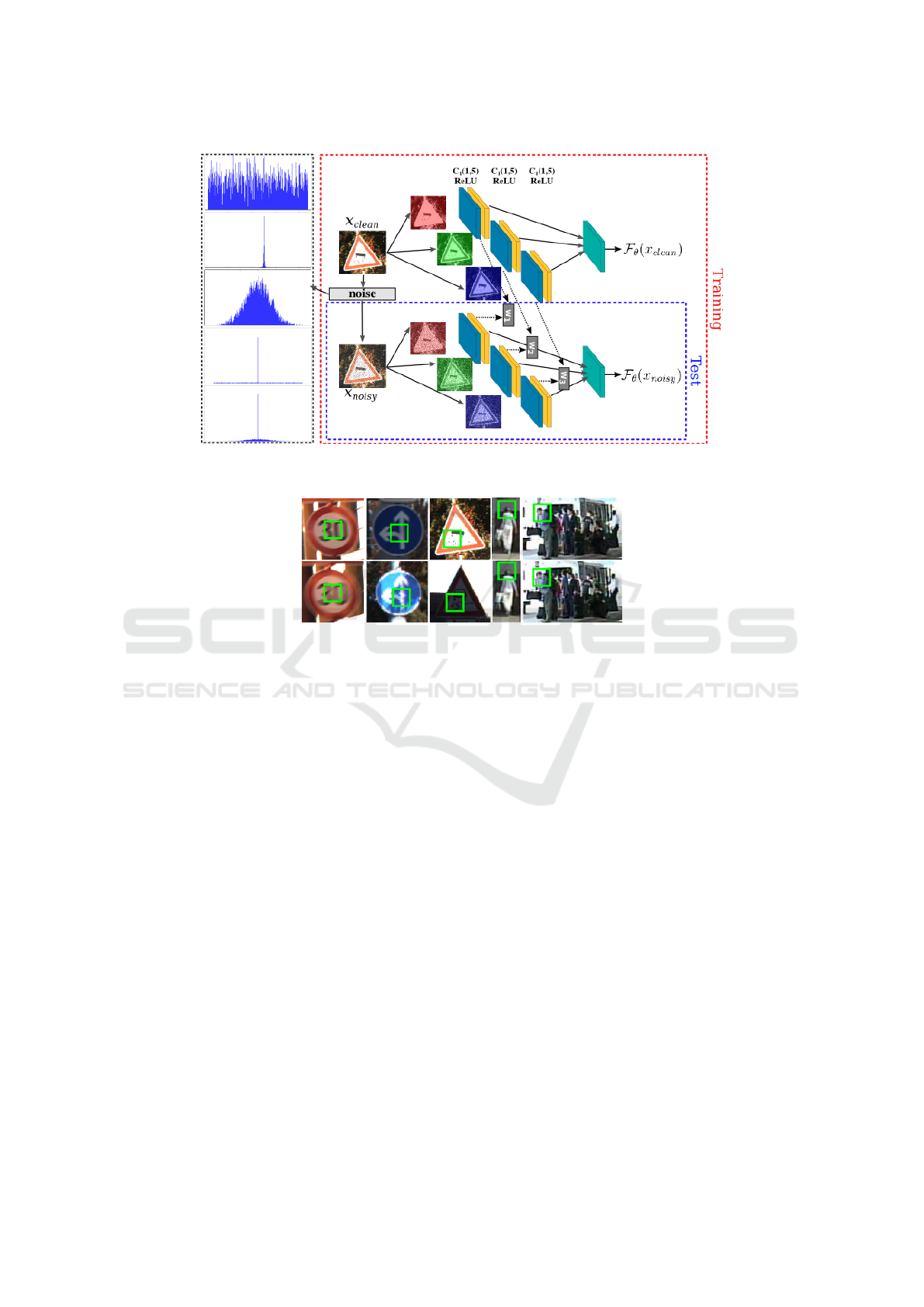
Figure 1: The proposed ConvNet for modelling F in (2). C(s, k) shows a convolution-ReLU layer containing s filters of size
k × k. Probability density function used for generating noise in the training phase is shown in the left.
Figure 2: Unclean training samples with contradictory patches (best viewed in color).
terms to our objective function. In terms of Lips-
chitz constant, the second term reduces the slope of
the hyperplane represented by each convolution ker-
nel. Moreover, it helps to reduce the effect of contra-
dictory patches.
4 EXPERIMENTS
We carry out our experiments on German Traffic Sign
Recognition Benchmark (GTSRB) (Stallkamp et al.,
2012) and Caltech-Pedestrian(Doll
´
ar et al., 2009)
datasets. The GTSRB and the Caltech-Pedestrian
datasets have some important characteristics. First,
they have been collected considering real scenarios
(e.g. shadow, lightening, occlusion, camera motion)
and they contain many degraded images. Second, the
imaging device are noisy and they produce artifacts
on the acquired images. Third, the resolution of im-
ages are low. Therefore, a slight change in the image
may affect the classification score.
We use 48 × 48 (the GTSRB dataset) and 64 × 64
(the Caltech-Pedestrian dataset) image patches as the
input of our layer. Also, we do not apply zero-padding
in the training phase to avoid the impact of border ef-
fect on the loss function. Besides, the input is nor-
malized to [0, 1]. All the weights in our layer are ini-
tialized using the normal distribution with mean value
set to 1 and standard deviation set to 0.2. Taking into
account the fact that each activation of the layer must
be in interval [0, 1], the initial weights are divided by
25 in order to make the results of convolution kernels
close to this interval. After we have the layer trained,
zero-padding is applied on the input.
Exploratory Analysis. To evaluate the restoration
accuracy of our method, we generate 150 noisy im-
ages for each sample in the test set. Generating a
noisy pattern is done in several steps. First, we ran-
domly select a uniform or a normal distribution with
probability 0.5. Then, a noisy pattern is generated
with µ = 0 and σ = U(0.5, 15) if the normal random
number generator is selected. Here, U (0.5, 15) re-
turns a number between 0.5 and 15 using the uniform
distribution. In the case of uniform random number
generator, the noisy pattern is generated in interval
[−3U(0.5, 15), 3U(0.5, 15)]. Next, the noisy pattern
is sparsified with probability 0.25. The sparsifica-
tion is done by generating a binary mask using bi-
nomial distribution with n = 1 and p = U (0.5, 1.0). It
is worth mentioning that we set the seed of random
Increasing the Stability of CNNs using a Denoising Layer Regularized by Local Lipschitz Constant in Road Understanding Problems
221

number generators to an identical value for all meth-
ods. Figure 3 illustrates a few noisy images along
with the noisy patterns generated on the GTSRB and
the Caltech-Pedestrian datasets.
The noisy samples are fed into the layer and the
peak signal to noise ratio of the restored image is
computed using the following equation:
psnr = 10 log
10
255
2
1
HW
∑
H
m=i
∑
W
n= j
(x − x
0
)
2
!
. (5)
In the above equation, x is the clean image and x
0
is
the noisy/restored image (both of them are re-scaled
back to [0, 255]). In addition, we also study how
the Lipschitz constant of our layer changes locally.
This is done by computing kF (x
i
clean
) − F (x
i
noisy
)k
and ν = kx
clean
− x
noisy
k. To compare our results with
other similar methods, we also restored the images
using the bilateral(d=5 and σ
1
= σ
2
= 9), the me-
dian(5 × 5) and Gaussian(5 × 5) filtering approaches.
Figure 4 illustrates the scatter plot of the PSNR study
(left) and the Lipschitz study (right) superimposed
with a polynomial fitted on the data.
According to the results, both Gaussian and me-
dian filtering approaches are not able to restore im-
age accurately. This is due to the fact that objects in
the GTSRB and the Caltech-Pedestrian datasets are
represented using low resolution images. On the one
hand, details of objects are mainly determined using
high frequency pixels. On the other hand, these pix-
els are close in the case of these low resolution im-
ages. As the result, Gaussian and median filtering ap-
proaches oversmooth the images which degrades the
edges of objects. For this reason, PSNR of the filtered
image is much lower than the PSNR of the noisy im-
age. In contrast, bilateral filtering preserves the edges
and this is the main reason that it has a higher PSNR
compared with these two methods. Moreover, bilat-
eral filtering restores image with higher PSNR when
the PSNR of the noisy image is less than 35.
The Lipschitz study shows that Gaussian and me-
dian filtering produce similar results regardless of the
magnitude of noise. In contrary, images restored by
bilateral filtering are scattered at a distance which is
approximately similar to the distance of the noisy im-
age from the clean image. We are looking for a fil-
tering approach which is able to restore images as ac-
curate as possible and it produces results with smaller
Lipschitz constant. Consequently, none of these three
approaches are appropriate for our purpose.
However, the filter learned by our approach has a
trade off between accuracy and the Lipschitz constant.
Looking at the PSNR values, we observe that, on av-
erage, it is more accurate than these three methods.
Besides, its Lipschitz constant is approximately lin-
ear. More importantly, the Lipschitz constant of our
filter is less than 1 which means that restored images
become closer after being filtered by our layer. Fi-
nally, we observe that the Lipschitz constant is very
stable with very low variation in our approach. This
means that, the filter learned by our objective function
is not sensitive to the variations of input image.
We further analyze our filters in the frequency do-
main using the Fourier transform. Figure 5 illustrates
the frequency response of our filters along with the
Gaussian filter. First, our filters have higher response
to low frequencies than the Gaussian filter. For this
reason, it passes some of the details in the image more
than Gaussian filter. Second, they also have higher re-
sponses in very high frequencies. This helps our fil-
ters to preserve edges more than the Gaussian filter.
Quantitative Analysis. We pick the ConvNet in (An-
gelova et al., 2015) for detecting pedestrians and the
ConvNet in (Aghdam et al., 2015) for classification
of traffic signs. First, these ConvNets are trained
on the GTSRB and the Caltech-Pedestrians datasets.
Then, we connect our learned restoration filters to
these ConvNets and fine-tune them for one epoch on
the original dataset (we do not augment the dataset
with noisy images). Then, the ConvNets are tested
using noisy test sets. We repeat this procedure (fine
tuning the classification ConvNets) on Gaussian, me-
dian and bilateral filtering as well.
The noisy test sets are created by generating 1050
Guassian noise pattern with σ ∈ {0.3, 1, 2, 3, 4, 8, 10}
for each sample (150 images per each value of σ).
Then, we feed these noisy samples to the above Con-
vNets (after connecting our layer to these ConvNets)
and compute the accuracy. To generate the same noisy
samples for all methods in our experiment, we always
seed the random number generator with a fixed value.
Table 1 and Table 2 show the results on the GTSRB
and the Caltech-Pedestrian datasets.
We observe that adding a Guassian or a me-
dian3x3 layer to the GTSRB ConvNet increases the
classification accuracy of the ConvNet on clean im-
ages. This is due to the fact that some of the test
samples might be noisy for the reasons we discussed
in Section 3. The Gaussian layer helps to deal with
this kind of noise and consequently it increases the
accuracy of the ConvNet on clean samples. Simi-
larly, median3x3 and bilateral1 filtering increases the
accuracy of the Caltech-Pedestrian ConvNet on clean
samples compared with the original ConvNet. How-
ever, while Gaussian filtering works well on the GT-
SRB dataset it does not increase the accuracy on the
Caltech-Pedestrian dataset. Likewise, bilateral filter-
ing improves the accuracy on the Caltech-Pedestrian
VISAPP 2017 - International Conference on Computer Vision Theory and Applications
222
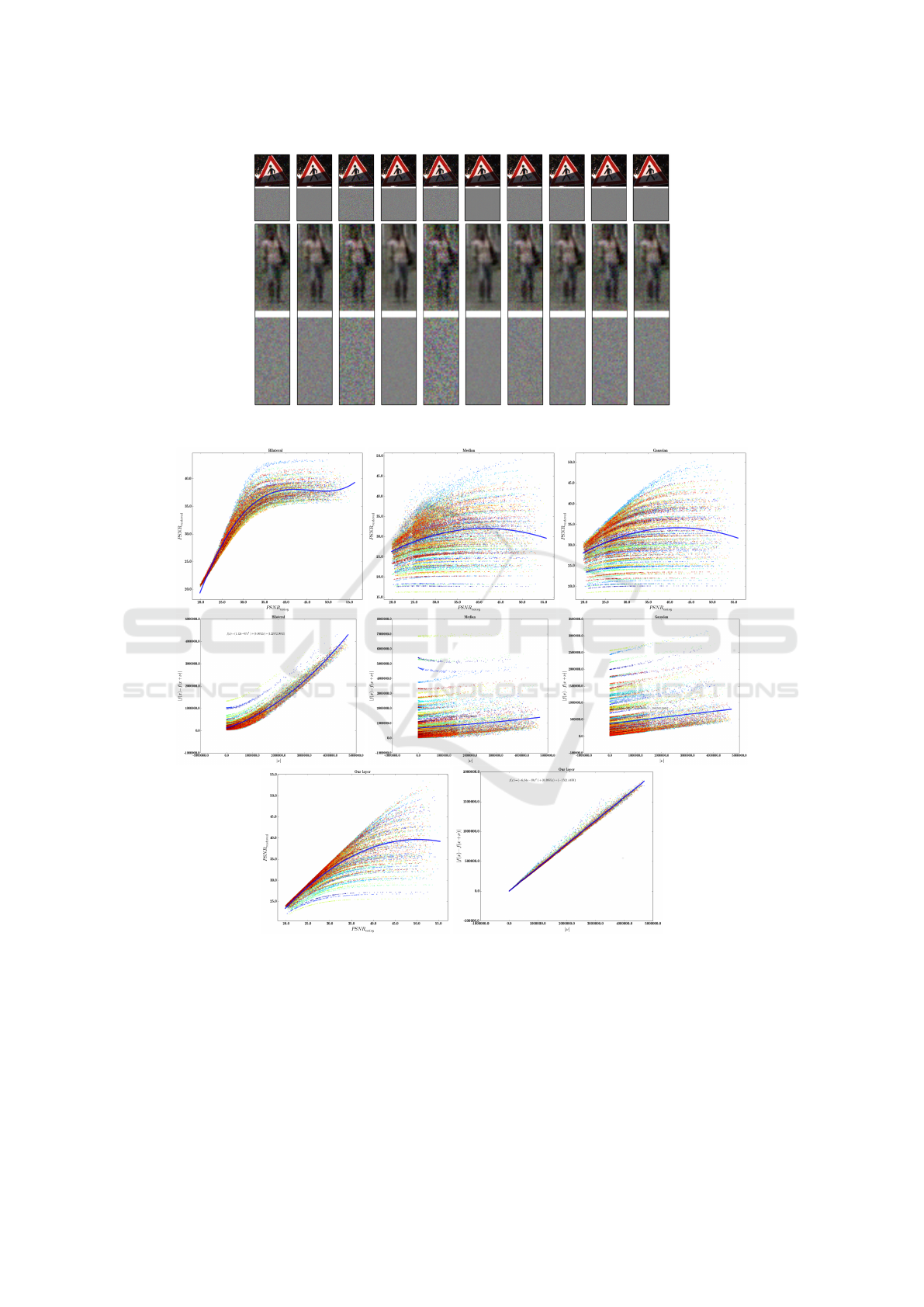
Figure 3: Samples of noisy images generated by our algorithm.
Figure 4: PSNR (left) and Lipschitz analysis (right) of the the Gaussian, median, bilateral and our approaches (best viewed in
color and electronically).
dataset but they do not increase the accuracy on the
GTSRB dataset.
Notwithstanding, the filters learned by our method
produce the most accurate results on both datasets. In
addition, our layer produce a ConvNet with highest
stability against noise compared with approaches with
similar computational complexity. In fact, the com-
putational complexity of our layer is identical to the
Gaussian 5x5 and its less than bilateral and median
filtering approaches.
Analyzing Results. Figure 6 illustrates some of the
samples that are classified incorrectly by the original
ConvNet but they are classified correctly after being
smoothed by our method. The original image inside
Increasing the Stability of CNNs using a Denoising Layer Regularized by Local Lipschitz Constant in Road Understanding Problems
223
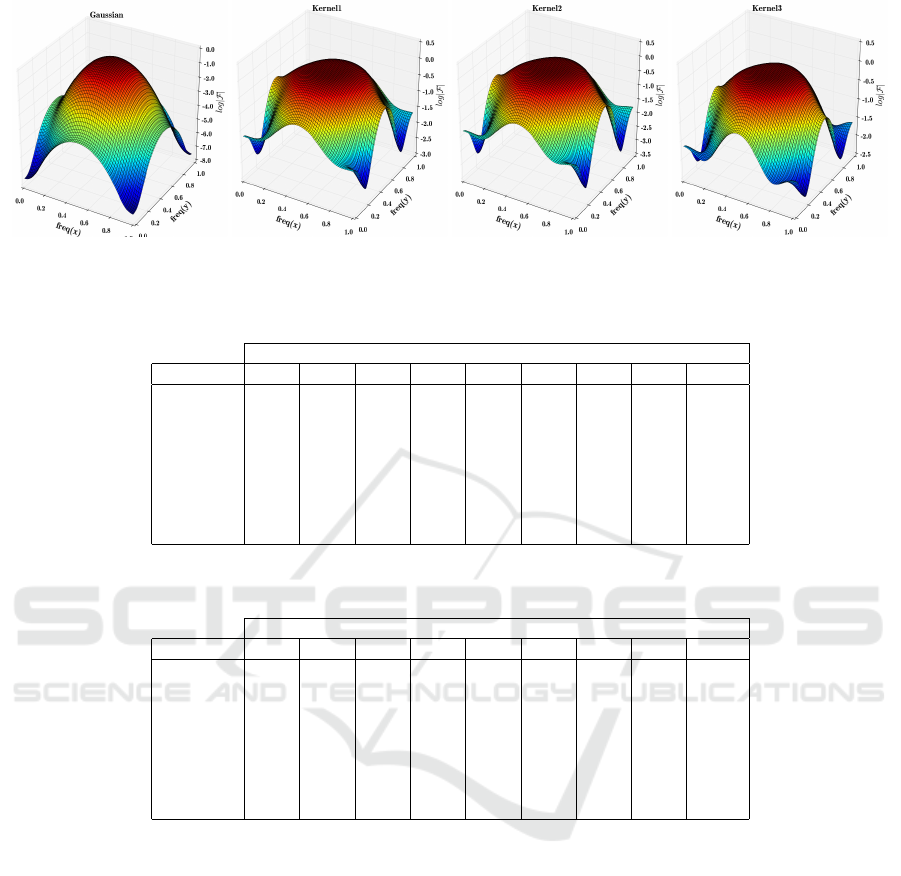
Figure 5: Comparing our filter with Gaussian filter in the frequency domain.
Table 1: Accuracy of the GTSRB ConvNet obtained by degrading the test images in the original dataset using a Gaussian
noise with various values of σ.
accuracy (%) for different values of σ
network clean 0.3 1 2 3 4 8 10 overall
original 99.06 98.56 98.56 98.55 98.52 98.48 98.20 97.93 98.48
gaussian3x3 99.22 98.72 98.72 98.71 98.68 98.64 98.36 98.13 98.65
gaussian5x5 99.22 98.71 98.71 98.70 98.68 98.65 98.42 98.23 98.66
median3x3 99.15 98.66 98.66 98.65 98.63 98.60 98.38 98.19 98.62
median5x5 98.94 98.42 98.42 98.39 98.36 98.32 98.04 97.83 98.34
bilateral1 98.99 98.49 98.49 98.48 98.46 98.45 98.27 98.13 98.47
bilateral2 96.94 96.49 96.48 96.48 96.44 96.42 96.28 96.17 96.46
our filter 99.31 99.31 99.31 99.30 99.28 99.26 99.03 98.84 99.21
Table 2: Accuracy of the Caltech-Pedestrian ConvNet obtained by degrading the test images in the original dataset using a
Gaussian noise with various values of σ.
accuracy (%) for different values of σ
network clean 0.3 1 2 3 4 8 10 overall
original 92.39 91.97 91.97 91.97 91.95 91.92 91.67 91.49 91.92
gaussian3x3 92.36 91.89 91.89 91.87 91.85 91.80 91.61 91.48 91.84
gaussian5x5 92.01 91.52 91.52 91.49 91.46 91.43 91.23 91.12 91.47
median3x3 92.61 92.16 92.16 92.16 92.17 92.16 92.07 92.02 92.19
median5x5 92.18 91.67 91.67 91.66 91.64 91.61 91.46 91.34 91.65
bilateral1 92.74 92.27 92.26 92.25 92.25 92.22 92.13 92.03 92.27
bilateral2 92.27 91.82 91.82 91.83 91.82 91.81 91.83 91.84 91.88
our filter 92.86 92.84 92.83 92.81 92.78 92.76 92.56 92.46 92.74
the green rectangle is degraded by shadow. Our layer
filters the edges of the object and reduces the effect
of shadow on the edges. The background of the im-
age inside the red rectangle is smoothed by the layer.
Edges in the original image inside the yellow rectan-
gle has Bayer like pattern because of excessive light-
ening in the background. This effect is reduced by our
filter. Finally, a general filtering is applied on the im-
age inside the blue rectangle and makes it smoother.
In sum, our method increases the accuracy by improv-
ing degraded edges and smoothing background noise.
5 CONCLUSION
In this paper, we proposed a lightweight approach for
increasing stability of ConvNets. Our method trains
a ReLU layer containing 3 channel-wise filters. We
proposed a new objective function consisting of the
sum of square error penalized by the Lipschitz con-
stant of the filters. We showed that the Lipschitiz con-
stant in this particular configuration act as an adap-
tive L
2
regularizer. Our experiments on the GTSRB
and the Caltech-Pedestrian datasets shows that this
approach increases the accuracy of the original Con-
vNets on the clean test sets. Using our approach, the
stability of ConvNets increases while the computa-
tional cost of our layer is negligible. Besides, since
it is a modular approach, we do not need to train a
large ConvNet using thousands of noisy samples to
increase the stability. Rather, we train the classifica-
tion ConvNet on the clean dataset. Then, we train
our restoration layer on the noisy training set. Finally,
the classification ConvNet is fine-tune for one epoch
using the clean training set. This approach is very af-
VISAPP 2017 - International Conference on Computer Vision Theory and Applications
224

Figure 6: Images that are correctly classified after being filtered by our layer. Left to right: Original image, difference with
restored, restored image and normalized difference.
fordable in terms of time and computation resources.
ACKNOWLEDGEMENTS
Hamed H. Aghdam and Elnaz J. Heravi are grateful
for the supports granted by Generalitat de Catalunya’s
Ag
`
ecia de Gesti
´
o d’Ajuts Universitaris i de Recerca
(AGAUR) through the FI-DGR 2015 fellowship and
University Rovira i Virgili through the Marti Franques
fellowship, respectively.
REFERENCES
Aghdam, H. H., Heravi, E. J., and Puig, D. (2015). Rec-
ognizing Traffic Signs using a Practical Deep Neural
Network. In Robot 2015: Second Iberian Robotics
Conference, pages 399–410, Lisbon. Springer.
Aghdam, H. H., Heravi, E. J., and Puig, D. (2016). Ana-
lyzing the Stability of Convolutional Neural Networks
Against Image Degradation. In Proceedings of the
11th International Conference on Computer Vision
Theory and Applications.
Alhussein Fawzi, Omar Fawzi, and Pascal Frossard (2015).
Analysis of classifiers’ robustness to adversarial per-
turbations. (2014):1–14.
Angelova, A., Krizhevsky, A., View, M., View, M., Van-
houcke, V., Ogale, A., and Ferguson, D. (2015). Real-
Time Pedestrian Detection With Deep Network Cas-
cades. Bmvc2015, pages 1–12.
Bittel, S., Kaiser, V., Teichmann, M., and Thoma, M.
(2015). Pixel-wise Segmentation of Street with Neural
Networks. pages 1–7.
Burger, H. C., Schuler, C. J., and Harmeling, S. Image
denoising Can plain neural networks compete with
BM3D .
Cirean, D., Meier, U., Masci, J., and Schmidhuber, J.
(2012). Multi-column deep neural network for traf-
fic sign classification. Neural Networks, 32:333–338.
Doll
´
ar, P., Wojek, C., Schiele, B., and Perona, P. (2009).
Pedestrian detection: A benchmark. 2009 IEEE Com-
puter Society Conference on Computer Vision and
Pattern Recognition Workshops, CVPR Workshops
2009, pages 304–311.
Dong, C., Loy, C. C., and He, K. (2014). Image
Super-Resolution Using Deep Convolutional Net-
works. arXiv preprint, 8828(c):1–14.
Goodfellow, I. J., Shlens, J., and Szegedy, C. (2015). Ex-
plaining and Harnessing Adversarial Examples. Iclr
2015, pages 1–11.
Gu, S. and Rigazio, L. (2014). Towards Deep Neural Net-
work Architectures Robust to Adversarial Examples.
arXiv:1412.5068 [cs], (2013):1–9.
He, K., Zhang, X., Ren, S., and Sun, J. (2015). Deep
Residual Learning for Image Recognition. In arXiv
prepring arXiv:1506.01497.
Hradi, M. (2015). Convolutional Neural Networks for Di-
rect Text Deblurring. Bmvc, (1):1–13.
Jain, V. and Seung, S. (2009). Natural Image Denoising
with Convolutional Networks. pages 769–776.
Krizhevsky, A., Sutskever, I., and Hinton, G. (2012). Im-
agenet classification with deep convolutional neural
networks. In Advances in neural information process-
ing systems, pages 1097–1105. Curran Associates,
Inc.
Levi, D., Garnett, N., and Fetaya, E. (2015). StixelNet: a
deep convolutional network for obstacle detection and
road segmentation. Bmvc, pages 1–12.
Papernot, N., McDaniel, P., Jha, S., Fredrikson, M., Celik,
Z. B., and Swami, A. (2015). The Limitations of Deep
Learning in Adversarial Settings.
Sabour, S., Cao, Y., Faghri, F., and Fleet, D. J. (2015).
Adversarial Manipulation of Deep Representations.
arXiv preprint arXiv:1511.05122, (2015):1–10.
Sermanet, P. and Lecun, Y. (2011). Traffic sign recognition
with multi-scale convolutional networks. Proceedings
of the International Joint Conference on Neural Net-
works, pages 2809–2813.
Simonyan, K. and Zisserman, A. (2015). Very Deep Con-
volutional Networks for Large-Scale Image Recogni-
tion. In International Conference on Learning Repre-
sentation (ICLR), pages 1–13.
Srivastava, R. K., Greff, K., and Schmidhuber, J. (2015).
Highway Networks. arXiv:1505.00387 [cs].
Stallkamp, J., Schlipsing, M., Salmen, J., and Igel, C.
(2012). Man vs. computer: Benchmarking machine
learning algorithms for traffic sign recognition. Neu-
ral Networks, 32:323–332.
Svoboda, P., Hradis, M., Marsik, L., and Zemcik, P. (2016).
CNN for License Plate Motion Deblurring.
Szegedy, C., Reed, S., Sermanet, P., Vanhoucke, V., and
Rabinovich, A. (2014a). Going deeper with convolu-
tions. In arXiv preprint arXiv:1409.4842, pages 1–12.
Szegedy, C., Zaremba, W., and Sutskever, I. (2014b). In-
triguing properties of neural networks.
Increasing the Stability of CNNs using a Denoising Layer Regularized by Local Lipschitz Constant in Road Understanding Problems
225
