Efficient Ray Traversal of Constrained Delaunay Tetrahedralization
Maxime Maria, S´ebastien Horna and Lilian Aveneau
University of Poitiers, XLIM, UMR 7252, Futuroscope Chasseneuil Cedex, Poitiers, France
Keywords:
Ray Tracing, Acceleration Structure, Constrained Delaunay Tetrahedralization.
Abstract:
Acceleration structures are mandatory for ray-tracing applications, allowing to cast a large number of rays per
second. In 2008, Lagae and Dutr´e have proposed to use Constrained Delaunay Tetrahedralization (CDT) as an
acceleration structure for ray tracing. Our experiments show that their traversal algorithm is not suitable for
GPU applications, mainly due to arithmetic errors. This article proposes a new CDT traversal algorithm. This
new algorithm is more efficient than the previous ones: it uses less arithmetic operations; it does not add extra
thread divergence since it uses a fixed number of operation; at last, it is robust with 32-bits floats, contrary to
the previous traversal algorithms. Hence, it is the first method usable both on CPU and GPU.
1 INTRODUCTION
Ray tracing is a widely used method in computer
graphics, known for its capacity to simulate com-
plex lighting effects to render high-quality realistic
images. However, it is also recognized as time-
consuming due to its high computational cost.
To speed up the process, many acceleration struc-
tures have been proposed in the literature. They are
often based on a partition of Euclidean space or ob-
ject space, like kd-tree (Bentley, 1975), BSP-tree,
BVH (Rubin and Whitted, 1980; Kay and Kajiya,
1986) and regular grid (Fujimoto et al., 1986). A
survey comparing all these structures can be found
in (Havran, 2000). They can reach interactive render-
ing, e.g exploiting ray coherency (Wald et al., 2001;
Reshetov et al., 2005; Mahovsky and Wyvill, 2006)
or GPU parallelization (Purcell et al., 2002; Foley
and Sugerman, 2005; G¨unther et al., 2007; Aila and
Laine, 2009; Kalojanov et al., 2011). Nevertheless,
actually a lot of factors impact on traversal efficiency
(scene layout, rendering algorithm, etc.).
A different sort of acceleration structures is the
constrained convex space partition (CCSP), slightly
studied up to then. A CCSP is a space partition into
convex volumes respecting the scene geometry. (For-
tune, 1999) introduces this concept by proposing a
topological beam tracing using an acyclic convexsub-
division respecting the scene obstacles, but using a
hand-made structure. Recently, (Maria et al., 2017)
present a CCSP dedicated to architectural environ-
ments, hence limiting its purpose. (Lagae and Dutr´e,
2008) propose to use a constrained Delaunay tetrahe-
dralization (CDT), i.e. CCSP only made up of tetrahe-
dra. However, our experiments show that their CDT
traversal methods cannot run on GPU, due to numer-
ical errors.
Using a particular tetrahedron representation, this
paper proposes an efficient CDT traversal, having the
following advantages:
• It is robust, since it does not cause any error due to
numerical instability, either on CPU or on GPU.
• It requires less arithmetic operations and so it is
inherently faster than previous solutions.
• It is adapted to parallel programming since it does
not add extra thread divergence.
This article is organized as follows: Section 2 re-
capitulates previous CDT works. Section 3 presents
our new CDT traversal. Section 4 discusses our ex-
periments. Finally, Section 5 concludes this paper.
2 PREVIOUS WORKS ON CDT
This section first describes CDT, then it presents its
construction from a geometric model, before focusing
on former ray traversal methods.
2.1 CDT Description
A Delaunay tetrahedralization of a set of points
X ∈ E
3
is a set of tetrahedra occupying the whole
236
Maria M., Horna S. and Aveneau L.
Efficient Ray Traversal of Constrained Delaunay Tetrahedralization.
DOI: 10.5220/0006131002360243
In Proceedings of the 12th International Joint Conference on Computer Vision, Imaging and Computer Graphics Theory and Applications (VISIGRAPP 2017), pages 236-243
ISBN: 978-989-758-224-0
Copyright
c
 2017 by SCITEPRESS – Science and Technology Publications, Lda. All rights reserved

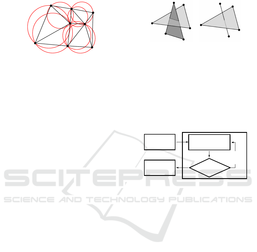
Figure 1: Delaunay triangulation: no vertex is inside a cir-
cumscribed circle.
space and respecting the Delaunay criterion (Delau-
nay, 1934): a tetrahedron T, defined by four vertices
V ⊂ X, is a Delaunay tetrahedron if it exists a circum-
scribed sphere S of T such as no point of X \ {V} is
inside S. Figure 1 illustrates this concept in 2D.
Delaunay tetrahedralization is “constrained” if it
respects the scene geometry. In other words, all the
geometric primitives are necessarily merged with the
faces of the tetrahedra making up the partition.
Three kinds of CDT exist: usual constrained
Delaunay tetrahedralization (Chew, 1989), conform-
ing Delaunay tetrahedralization (Edelsbrunner and
Tan, 1992) and quality Delaunay tetrahedraliza-
tion (Shewchuk, 1998). In ray tracing context, (Lagae
and Dutr´e, 2008) proved that quality Delaunay tetra-
hedralization is the most efficient to traverse.
2.2 CDT Construction
CDT cannot be built from every geometric models. A
necessary but sufficient condition is that the model is a
piecewise linear complex (PLC) (Miller et al., 1996).
In 3D, any non empty intersection between two faces
of a PLC must correspond to either a shared edge or
vertex. In other words, there is no self-intersection
(Figure 2). In computer graphics, a scene is gener-
ally represented as an unstructured set of polygons. In
such a case, some self-intersections may exist. Nev-
ertheless, it is still possible to construct PLC using a
mesh repair technique such as (Zhou et al., 2016).
CDT can be built from a given PLC using the
Si’s method (Si, 2006). It results in a tetrahedral
mesh, containing two kinds of faces: occlusive faces,
belonging to the scene geometry; and some non-
occlusive faces, introduced to build the partition. Ob-
viously, a given ray should traverse the latter, as non-
occlusive faces do not belong to the input geometry.
2.3 CDT Traversal
Finding the closest intersection between a ray and
CDT geometry is done in two main steps. First, the
(a) (b)
Figure 2: Examples of two non-PLC configurations: inter-
section between (a) two faces, (b) an edge and a face.
tetrahedron containing the ray origin is located. Sec-
ond, the ray goes through the tetrahedralization by
traversing one tetrahedron at a time until hitting an
occlusive face. This process is illustrated in Figure 3.
Let us notice that there is no need to explicitly test
intersections with the scene geometry, as usual ac-
celeration structures do. This is done implicitly by
searching the exit face from inside a tetrahedron.
Locate
origin
Exit face search
Return
intersection
Occlusive
face?
Propagate
ray
CDT Traversal
Yes No
Figure 3: CDT traversal overview: the main key of any
CDT traversal algorithm lies in the “exit face search” part.
2.3.1 Locating Ray Origin
Using pinhole camera model, all primary rays start
from the same origin. For an interactive application
locating this origin is needed only for the first frame,
hence it is a negligible problem. Indeed, camera mo-
tion generally corresponds to a translation, for in-
stance when the camera is shifted, or when ray origins
are locally perturbed for depth-of-field effect. Using a
maximal distance in the traversal algorithm efficiently
solves this kind of move.
Locating the origin of non primary rays is avoided
by exploiting implicit ray connectivity inside CDT:
both starting point and volume correspond to the ar-
rival of the previous ray.
2.3.2 Exit Face Search
Several methods have been proposed in order to find
the exit face of a ray from inside a tetrahedron. (La-
gae and Dutr´e, 2008) present four different ones. The
first uses four ray/plane intersections and is similar to
(Garrity, 1990). The second is based on half space
classification. The third finds the exit face using 6
Efficient Ray Traversal of Constrained Delaunay Tetrahedralization
237

permuted inner products (called side and noted ⊙) of
Pl¨ucker coordinates (Shoemake, 1998). It is similar to
(Platis and Theoharis, 2003) technique. Their fourth
and fastest method uses 3 to 6 Scalar Triple Products
(STP). It is remarkable that none of these four meth-
ods exploits the knowledge of the ray entry face.
For volume rendering, (Marmitt and Slusallek,
2006) extend (Platis and Theoharis, 2003). Their
method (from now MS06) exploits neighborhood re-
lations between tetrahedra to automatically discard
the entry face. It finds the exit face using 2,67 side
products on average. Since the number of products
varies, MS06 exhibits some thread divergence in par-
allel environment. This drawback also appears with
the fastest Lagae et al. method.
All these methods are not directly usable on GPU,
due to numerical instability. Indeed, the insufficient
arithmetic precision with 32-bits floats causes some
failures to traverse CDT, leading to infinite loops.
In this paper, we propose a new traversal algo-
rithm, based on Pl¨ucker coordinates. Like MS06,
it exploits the neighborhood relations between faces.
The originality lies in our specific tetrahedron repre-
sentation, allowing to use exactly 2 optimized side
products.
3 NEW TRAVERSAL
ALGORITHM
CDT traversal algorithm is a loop, searching for the
exit face from inside a tetrahedron (Figure 3). We
propose a new algorithm, both fast and robust. It
uses Pl¨ucker coordinates, i.e. six coordinates corre-
sponding to the line direction u and moment v. Such
a line is oriented: it passes through a first point p, and
then a second one q. Then, u = q− p and v = p × q.
For two lines l = {u : v} and l
′
= {u
′
: v
′
}, the sign
of the side product l ⊙ l
′
= u · v
′
+ v· u
′
indicates the
relative orientation of the two lines: negative value
means clockwise orientation, zero value indicates in-
tersection, and positive value signifies counterclock-
wise orientation (Shoemake, 1998).
3.1 Exit Face Search
Our algorithm assumes that the entry face is known,
and that the ray stabs the current tetrahedron. For a
given entry face, we use its complementin the tetrahe-
dron, i.e. the part made of one vertex, three edges and
three faces. We denote Λ
0
, Λ
1
and Λ
2
the complement
edges, with counterclockwise orientation from inside
the tetrahedron (Figure 4). We number complement
faces with a local identifier from 0 to 2, such that:
Λ
2
Λ
0
Λ
1
r
r⊙ Λ
1
r⊙ Λ
2
21
< 0
≥ 0 ≥ 0
r⊙ Λ
0
< 0< 0
≥ 0
1
0
(b)(a)
Figure 4: Exit face search example: (a) ray r enters the
tetrahedron through the back face; (b) r ⊙ Λ
2
< 0 and r ⊙
Λ
0
≥ 0, so the exit face is identified by 0.
face 0 is bounded by Λ
0
and Λ
2
, face 1 is bounded
by Λ
1
and Λ
0
, and face 2 is bounded by Λ
2
and Λ
1
.
Using Pl¨ucker side product, the face stabbed by ray r
is:
• face 0, if and only if r turns counterclockwise
around Λ
0
and clockwise around Λ
2
(r ⊙ Λ
0
≥ 0
and r⊙ Λ
2
< 0);
• face 1, if and only if r turns counterclockwise
around Λ
1
and clockwise around Λ
0
(r ⊙ Λ
1
≥ 0
and r⊙ Λ
0
< 0);
• face 2, if and only if r turns counterclockwise
around Λ
2
and clockwise around Λ
1
(r ⊙ Λ
2
≥ 0
and r⊙ Λ
1
< 0).
We compact these conditions into a decision tree
(Figure 4(b)). Each leaf corresponds to an exit face,
and each interior node represents a side product
between r and a line Λ
i
. At the root, we check r⊙Λ
2
.
If it is negative (clockwise), then r cannot stab face
2: in the left subtree, we only have to determine
if r stabs face 0 or 1, using their shared edge Λ
0
.
Otherwise, r turns counterclockwise around Λ
2
and
so cannot stab face 0, and the right subtree we check
if r stabs face 1 or 2 using their shared edge Λ
1
.
With Figure 4(a) example, r turns clockwise around
Λ
2
and then counterclockwise around Λ
0
; so, r exits
through face 0.
Algorithm 1: Exit face search from inside a tetrahedron.
Require: F
e
= {Λ
0
, Λ
1
, Λ
2
}: entry face; Λ
r
: ray;
Ensure: F
s
: exit face;
1: side ← Λ
r
⊙ F
e
.Λ
2
;
2: id ← (side ≥ 0); {id ∈ {0, 1}}
3: side ← Λ
r
⊙ F
e
.Λ
id
;
4: id ← id + (side < 0); {id ∈ {0, 1, 2}}
5: F
s
← getFace(F
e
,id);
6: return F
s
;
GRAPP 2017 - International Conference on Computer Graphics Theory and Applications
238

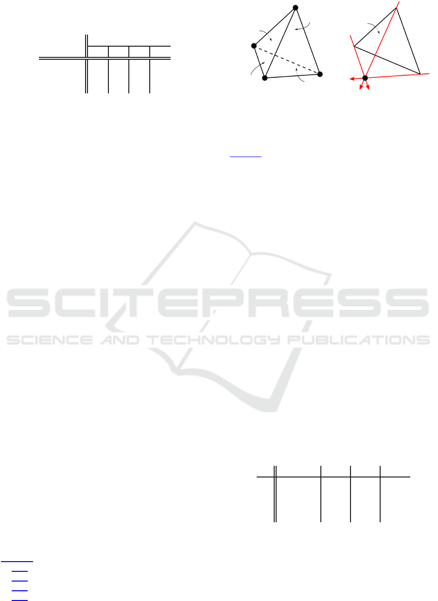
Table 1: Exit face according to the entry face and a local
identifier in {0, 1, 2}, following a consistent face numbering
(Figure 5(a)).
Exit
Entry face
identifier F
0
F
1
F
2
F
3
0 F
1
F
0
F
0
F
0
1
F
2
F
3
F
1
F
2
2 F
3
F
2
F
3
F
1
Since every decision tree branch has a fixed depth
of 2, our new exit face search method answers using
exactly two side products. Moreover, it is optimized
to run efficiently without any conditional instruction
(Algorithm 1). Notice that leave labels form two pairs
from left to right: the first pair (0,1) is equal to the
second (1,2), minus 1. Then, it uses that successful
logical test returns 1 (and 0 in failure case) to decide
which face to discard. So, the test r ⊙ Λ
2
≥ 0 allows
to decide if we have to consider the first or the second
pair. Finally, the same method is used with either the
line Λ
0
or Λ
1
.
This algorithm ends with
getFace function call.
This function returns the tetrahedron face number ac-
cording to the entry face and to the exit face label.
It answers using a lookup-table, defined using simple
combinatorics (Table 1), assuming a consistent label-
ing of tetrahedron faces (Figure 5(a)).
3.2 Data Structure
Algorithm 1 works for any entry face of any tetrahe-
dron. It relies on two specific representations of the
tetrahedron faces: a local identifier in {0, 1, 2}, and
global face F
i
, i ∈ [0. . . 3]. For a given face, it uses 3
Pl¨ucker lines Λ
i
. Since such lines contain 6 coordi-
nates, a face needs 18 single precision floats for the
lines (18 × 32 bits), plus brdf and neighborhood data
(tetrahedron and face numbers).
To reduce data size and balance GPU computa-
tions and memory accesses, we dynamically calculate
the Pl¨ucker lines knowing their extremities: each line
starts from a face vertex and ends with the comple-
ment vertex. So, we need all the tetrahedron vertices.
We arrange the faces such that their complement ver-
tex have the same number, implicitly known. Vertices
are stored into tetrahedra (for coalescent memory ac-
cesses), and vertex indices (in [0. . . 3]) are stored into
faces. This leads to the following data structure:
st ru ct Face {
in t br df ; / / −1: Non−Occlusive
in t t e t r a ; / / neighbor
in t f ace ; / / neighbor
in t idV [ 3 ] ; / / face v e r t i c e s
} ;
V
3
V
2
V
1
V
0
F
1
F
0
F
2
F
3
(a)
V
3
F
3
Λ
2
Λ
0
Λ
1
(b)
Figure 5: Description of a tetrahedron: (a) vertices and
faces numbering; (b) the complement vertex for F
3
is {V
3
},
and its edges are Λ
0
= V
1
V
3
, Λ
1
= V
0
V
3
and Λ
2
= V
2
V
3
.
st ru ct T etrahedron {
f l o a t 3 V[ 4 ] ;
/ / v e r t i c e s
Face F [ 4 ] ; / / f a c es
} ;
To save memory and so bandwidth, we compact
the structure Face . The neighboring face (the field
face ) is a number between 0 and 3; it can be encoded
using two bits, and so packed with the field tetra ,
corresponding to the neighboring tetrahedron. Thus,
tetrahedron identifiers are encoded on 30 bits, allow-
ing a maximum of one billion tetrahedra. In a similar
way, field
idV needs only 2 bits per vertex. But, they
are common to all the tetrahedra, and so are stored
only once for all into 4
unsigned char . Hence, a
face needs 8 bytes, and a full tetrahedron 80 bytes.
Notice that, on GPU a vertex is represented by 4 floats
to have aligned memory accesses. Then on GPU a full
tetrahedron needs 96 bytes.
Figure 5 proposes an example: for F
3
(made using
the complement vertex V
3
and counterclockwise ver-
texes V
1
, V
0
and V
2
), we can deduce that Λ
0
= V
1
V
3
,
Λ
1
= V
0
V
3
and Λ
2
= V
2
V
3
. Table 2 gives the descrip-
tion of faces according to their vertices and edges, fol-
lowing face numbering presented in Figure 5(a).
Table 2: Complement edges of entry face F
i
are implicitly
described by the face complement vertex (identified by i),
and its vertices in counterclockwise order.
F
Vertexes Λ
0
Λ
1
Λ
2
0 {3, 1, 2} V
3
V
0
V
1
V
0
V
2
V
0
1 {2, 0, 3} V
2
V
1
V
0
V
1
V
3
V
1
2
{3, 0, 1} V
3
V
2
V
0
V
2
V
1
V
2
3 {1, 0, 2} V
1
V
3
V
0
V
3
V
2
V
3
3.3 Exiting the Starting Volume
Algorithm 1 assumes known the entry face. This con-
dition is not fulfilled for the starting tetrahedron. Al-
gorithm 1 must be adapted in that case. A simple so-
lution lies in using a decision tree of depth 4, leading
Efficient Ray Traversal of Constrained Delaunay Tetrahedralization
239

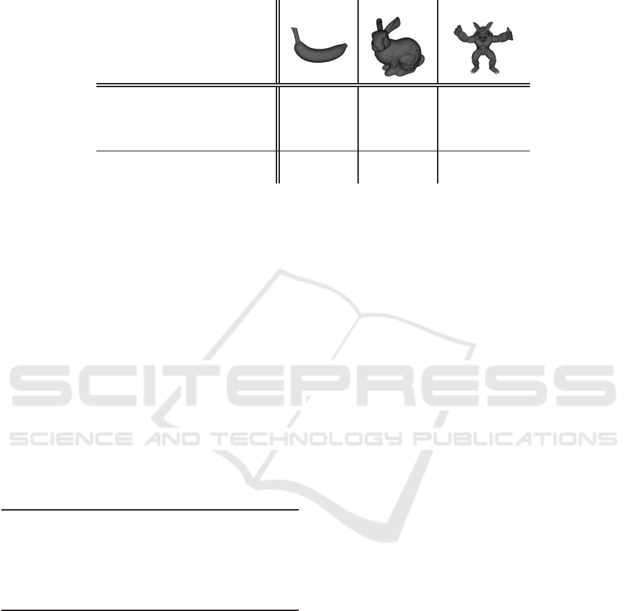
Table 3: Scenes characteristics and performance: number of tetrahedra, number of occlusive faces (faces coming from the
model), number of non-occlusive faces (faces created during tetrahedralization), occupied memory and ray casting perfor-
mance in millions of ray cast per second on CPU and GPU.
BANANA BUNNY ARMADILLO
Tetrahedra 71,300 682,733 2,990,552
Occlusive faces 24,568 222,775 1,105,218
Non-occlusive faces
117,994 1,142,650 4,875,834
Memory (MB) 6 62 273
Ray-casting (Mray/s)
CPU
9.76 10.5 6.75
GPU
428 289 123
to three Pl¨ucker side products. One can settle this tree
starting with any edge to discriminate between two
faces, and so on with the children.
Nevertheless, a simpler but equivalent solution
exists. Once the root fixed, we have only three
possible exit faces. This corresponds to Algorithm 1,
as if the discarded face was the entry one. So, we
just choose one edge to discard a face and then we
call Algorithm 1 with the discarded exit face as
the fake entry one. This leads to Algorithm 2. We
naturally choose edge V
2
V
3
shared by faces F
0
and F
1
(Figure 5(a)). If the side product is negative, then we
cannot exit through F
1
. Else, with a positive or null
value, we cannot exit through F
0
. Thus, the starting
tetrahedron problem is solved using three and only
three side products.
Algorithm 2: Exit face search from the starting tetrahedron.
Require: T = {V
i
, F
i
}
i∈[0...3]
: Tetrahedron; Λ
r
: Ray;
Ensure: F
s
: exit face;
1: side ← Λ
r
⊙V
2
V
3
;
2: f← side < 0; {f∈ {0, 1}}
3: return ExitTetra(F
f
, Λ
r
); {Algorithm 1}
3.4 Efficient Side Product
Both Algorithm 1 and 2 use Pl¨ucker side products. A
naive approach results in 23 operations per side prod-
uct: to calculate Pl¨ucker coordinates, we need 3 sub-
tractions for its direction and 6 multiplications and 3
subtractions for its moment. Then, side product needs
6 multiplications and 5 additions. The two side prod-
ucts in Algorithm 1 result in 46 operations.
We propose a new method using less operations. It
rests upon a coordinate system translation to the com-
plement vertex V
f
of the entry face. In this local sys-
tem, lines Λ
i
have a nil moment (since they contain
the origin). So, side products are inner products of
vectors having only 3 coordinates: each one needs 3
multiplications and 2 additions. Moreover, line direc-
tions are computed using 3 subtractions. Hence, such
side products need only 8 operations.
Nevertheless, we also need to modify Pl¨ucker co-
ordinates of the ray r to obtain valid side products.
Let us recall how a Pl¨ucker line is made. We com-
pute its direction u using two points p and q on the
line, and its moment v with p × q = p × u. In the lo-
cal coordinates system, the new line coordinates must
be calculated using translated points. The direction is
obviously the same, only v is modified:
v
′
= (p−V
f
) × u
= p× u−V
f
× u
= v−V
f
× u.
So, v
′
is calculated using 12 operations: 3 subtrac-
tions, 6 multiplications and 3 subtractions. This ray
transformation is done once per tetrahedron, the local
coordinates system being shared for all the lines Λ
i
.
As a conclusion, the number of arithmetic opera-
tions involved in Algorithm 1 can be decreased from
46 to 28, saving about 40% of computations.
4 EXPERIMENTS
This section discusses some experiments made using
our new traversal algorithm.
4.1 Results
Performance is evaluated using three objects tetrahe-
dralized using Tetgen (Si, 2015). Table 3 sums up
their main characteristics and measured performance.
The simplest object is constructed from a banana
GRAPP 2017 - International Conference on Computer Graphics Theory and Applications
240

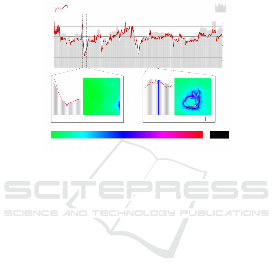
T = 40.1 ms - Φ = 9.6
(A)
T = 122 ms - Φ = 22.71
(B)
Φ
T
200
160
120
80
40
0
35
30
25
20
15
0
10
5
1000 200
Number of traversed tetrahedra per ray
200+
Figure 6: Rendering times on CPU in ms (T, red curve) and number of traversed tetrahedra in millions (Φ, gray bars) using
1,282 points of view and BUNNY; (A) T = 40.1 ms - Φ = 9.6; (B) T = 122 ms - Φ = 22.71.
model, with 25k occlusive faces. The other two corre-
spond to well-known Stanford’s objects: BUNNY and
ARMADILLO. Their CDT respectively count 200k
and 1.1M occlusive faces. We use quality CDT, in-
troducing new vertices into object models, explaining
the high number of faces our three objects have.
Performance is measured in millions of ray cast
per second (Mrays/s) using ray casting, 1024 × 1024
pixels and no anti-aliasing. The used computer pos-
sesses an Intel
R

Core
TM
i7-4930K CPU @ 3.40Ghz,
32 Gb RAM and NVidia
R

GeForce
R

GTX 680. Al-
gorithms are made parallel on CPU (OpenMP) and
GPU (CUDA, with persistent threads (Aila et al.,
2012)). On average, CPU ray casting reaches 9
Mrays/s, GPU version 280 Mrays/s.
4.2 Traversal
Closest ray/object intersection is found by traversing
CDT one tetrahedron at a time until hitting an occlu-
sive face. The ray traversal complexity is linear in
the number of traversed tetrahedra. Figure 6 shows
the relation between execution time (T) and number
of traversed tetrahedra per image (Φ). Statistics are
extracted on CPU using 1,282 points of view from
BUNNY.
The execution time is proportional to Φ: on point
of view (A), almost 10 millions tetrahedra are tra-
versed in 40.1 ms; on point of view (B), we tra-
verse 23 millions tetrahedra in 122 ms. It is not
strictly proportional, mainly due to memory accesses
that become more important when more tetrahedra
are traversed, leading to more memory cache defaults.
False-colored image of point of view (B) reveals that
rays going close to object boundary traverse more
tetrahedra.
4.3 Numerical Robustness
Using floating-point numbers can cause errors due to
numerical instability. Tetgen uses geometric predi-
cates (e.g. (Shewchuk, 1996) or (Devillers and Pion,
2003)) to construct robust CDT. If this is common
practice in algebraic geometry, it is not the case in
rendering. Hence, it is too expensive to be used in
CDT ray traversal.
We experimented three methods proposed in (La-
gae and Dutr´e, 2008) (ray/plane intersection tests,
Pl¨ucker coordinates and STP), plus the method pro-
posed in (Marmitt and Slusallek, 2006) (MS06) (Sec-
tion 2.3.2). We noticed they all suffer from numer-
ical errors either on CPU or GPU. Indeed, calcula-
tion are not enough precise with rather flat tetrahedra.
Thus, without extra treatment (like moving the ver-
tices) these algorithms may return a wrong exit face
or do not find any face at all (no test is valid). Table 4
reports for each object the number of rays per image
concerned by this problem, averaged over points of
view series.
In contrast, we did not obtain wrong results us-
Efficient Ray Traversal of Constrained Delaunay Tetrahedralization
241

Table 4: Numerical errors impact on GPU: number of rays
suffering from wrong results for 1024 × 1024 pixels, and
averaged over about 1, 300 points of view.
BANANA BUNNY ARMADILLO
Ray/plane 33.27 40.85 74.85
Pl¨ucker
3.6 22.25 412.13
STP 63.07 204.89 456.65
MS06
0.0007 0.004 0.422
Ours 0 0 0
ing our method. It can be explained by the smaller
number of performed arithmetic operations; less nu-
merical errors accumulated, more accurate results.
4.4 Exit Face Search Comparison
This section compares performance of our exit face
search algorithm with the same 4 previous methods:
ray/plane intersection tests, Pl¨ucker coordinates, STP
and MS06 (Section 2.3.2). Statistics are summed up
in Table 5. Times are measured for 16,384 random
rays stabbing 10,000 random tetrahedra, both on CPU
(using one thread) and GPU.
Table 5: Exit face search comparison: time (in ms) to deter-
mine the exit face for 10,000 tetrahedra and 16,384 random
rays per tetrahedron; on CPU (single thread) and on GPU.
Method
Time (ms)
CPU GPU
Ray/plane 15,623 36
Pl¨ucker 10,101 28
STP
4,876 29
MS06 5,994 21
Ours 2,663 13
CPU results show that our method is much more
efficient than former ones. This behavior is expected
since our new method requires less arithmetic opera-
tions. STP is the fastest previous method, but is 83%
slower than ours.
On GPU, results are slightly different. For exam-
ple, Pl¨ucker method is faster than STP. Indeed, even
if it requires more operations, it does not add extra
thread divergence. Hence, it is more adapted to GPU.
Among the previous GPU methods, the most efficient
is MS06, still 59% slower than ours.
4.5 State-of-the-art Comparison
In (Lagae and Dutr´e, 2008), authors noticed that ren-
dering using CDT as acceleration structure takes two
to three more computation times than using kdtree. In
this last section, we check if it is still the case using
our new tetrahedron exit algorithm and on GPU. We
Table 6: Performance comparison with (Aila et al., 2012),
in number of frames per second.
CDT
BVH
(Aila et al., 2012)
BANANA 315-947 200-260
BUNNY 130-1040 160-260
ARMADILLO
82-160 130-260
compare our GPU ray-tracer with the state-of-the-art
ray tracer (Aila et al., 2012), always using the same
computer. Their acceleration structure is BVH, con-
structed using SAH (MacDonald and Booth, 1990)
and split of large triangles (Ernst and Greiner, 2007).
To our knowledge, nowadays their implementation is
the fastest GPU one.
Table 6 sums up this comparison. Results show
that CDT is still not a faster acceleration structure
than classical ones (at least than BVH on GPU). First,
the timings show larger amplitude using CDT than
BVH. Moreover, while CDT is on average faster than
BVH with BANANA and BUNNY models, it is no
more true using ARMADILLO. This is directly linked
to the traversal complexity of the two structures. BVH
being built up following SAH, its performance is less
impacted with the geometry input size, contrary to
CDT where this size has a direct impact on perfor-
mance. Clearly, a heuristics similar to SAH is missing
for tetrahedralization.
5 CONCLUSION
This article proposes a new CDT ray traversal algo-
rithm. It is based upon a specific tetrahedron repre-
sentation, and fast Pl¨ucker side products. It uses less
arithmetic operations than previous methods. Last but
not least, it does not involve any conditional instruc-
tions, employing two and only two side products to
exit a given tetrahedron.
This algorithm exhibits several advantages com-
pared to the previous ones. Firstly it is inherently
faster, requiring less arithmetic operations. Secondly
it is more adapted to parallel computing, since having
a fixed number of operations it does not involve extra
thread divergence. Finally, it is robust and works with
32-bits floats either on CPU or GPU.
As future work, we plan to design a new construc-
tion heuristic, to obtain as fast to traverse as possible
CDT. Indeed, CDT traversal speed highly depends on
its construction. CDT traversal complexity is linear
in the number of traversed tetrahedra: the less tra-
versed tetrahedra, the more high performance. Be-
fore SAH introduction, the same problem existed with
well-known acceleration structures like kd-tree and
GRAPP 2017 - International Conference on Computer Graphics Theory and Applications
242

BVH, for which performance highly depends on the
geometric model. Since CDT for ray-tracing is a re-
cent method, we expect that similar heuristics exists.
REFERENCES
Aila, T. and Laine, S. (2009). Understanding the Efficiency
of Ray Traversal on GPUs. In High-Performance
Graphics, HPG ’09, pages 145–149.
Aila, T., Laine, S., and Karras, T. (2012). Understanding
the efficiency of ray traversal on GPUs – Kepler and
Fermi addendum. Technical report, NVIDIA Corp.
Bentley, J. L. (1975). Multidimensional Binary Search
Trees Used for Associative Searching. Communica-
tions of the ACM, 18(9):509–517.
Chew, L. P. (1989). Constrained Delaunay triangulations.
Algorithmica, 4:97–108.
Delaunay, B. (1934). Sur la sph`ere vide.
`
A la m´emoire de
Georges Vorono¨ı. Bulletin de l’Acad´emie des Sciences
de l’URSS, (6):793–800.
Devillers, O. and Pion, S. (2003). Efficient Exact Ge-
ometric Predicates for Delaunay Triangulations. In
5th Workshop on Algorithm Engineering and Exper-
iments, ALENEX ’03, pages 37–44.
Edelsbrunner, H. and Tan, T. S. (1992). An upper bound
for conforming delaunay triangulations. In 8th An-
nual Symposium on Computational Geometry, SCG
’92, pages 53–62.
Ernst, M. and Greiner, G. (2007). Early Split Clipping for
Bounding Volume Hierarchies. In IEEE Symposium
on Interactive Ray Tracing, RT ’07, pages 73–78.
Foley, T. and Sugerman, J. (2005). KD-tree Accelera-
tion Structures for a GPU Raytracer. In ACM SIG-
GRAPH/EUROGRAPHICS conference on Graphics
Hardware, HWWS ’05, pages 15–22.
Fortune, S. (1999). Topological Beam Tracing. In 15th An-
nual Symposium on Computational Geometry, SCG
’99, pages 59–68.
Fujimoto, A., Tanaka, T., and Iwata, K. (1986). ARTS:
Accelerated Ray-Tracing System. IEEE Computer
Graphics and Applications, 6(4):16–26.
Garrity, M. P. (1990). Raytracing Irregular Volume Data.
ACM SIGGRAPH Computer Graphics, 24(5):35–40.
G¨unther, J., Popov, S., Seidel, H.-P., and Slusallek, P.
(2007). Realtime Ray Tracing on GPU with BVH-
based Packet Traversal. In IEEE Symposium on Inter-
active Ray Tracing 2007, RT ’07, pages 113–118.
Havran, V. (2000). Heuristic Ray Shooting Algorithms.
PhD thesis, Department of Computer Science and En-
gineering, Faculty of Electrical Engineering, Czech
Technical University in Prague.
Kalojanov, J., Billeter, M., and Slusallek, P. (2011). Two-
Level Grids for Ray Tracing on GPUs. Computer
Graphics Forum, 30(2):307–314.
Kay, T. L. and Kajiya, J. T. (1986). Ray Tracing Com-
plex Scenes. ACM SIGGRAPH Computer Graphics,
20(4):269–278.
Lagae, A. and Dutr´e, P. (2008). Accelerating Ray Trac-
ing using Constrained Tetrahedralizations. Computer
Graphics Forum, (4):1303–1312.
MacDonald, D. J. and Booth, K. S. (1990). Heuristics for
Ray Tracing Using Space Subdivision. The Visual
Computer, 6(3):153–166.
Mahovsky, J. and Wyvill, B. (2006). Memory-Conserving
Bounding Volume Hierarchies with Coherent Raytrac-
ing. Computer Graphics Forum, 25(2):173–182.
Maria, M., Horna, S., and Aveneau, L. (2017). Constrained
Convex Space Partition for Ray Tracing in Architec-
tural Environments. Computer Graphics Forum.
Marmitt, G. and Slusallek, P. (2006). Fast Ray Traversal
of Tetrahedral and Hexahedral Meshes for Direct Vol-
ume Rendering. In 8th Joint EG / IEEE VGTC Confer-
ence on Visualization, EUROVIS ’06, pages 235–242.
Miller, G. L., Talmor, D., Teng, S.-H., Walkington, N.,
and Wang, H. (1996). Control Volume Meshes using
Sphere Packing: Generation, Refinement and Coars-
ening. In 5th International Meshing Roundtable, IMR
’96, pages 47–62.
Platis, N. and Theoharis, T. (2003). Fast Ray-Tetrahedron
Intersection Using Plucker Coordinates. Journal of
Graphics Tools, 8(4):37–48.
Purcell, T. J., Buck, I., Mark, W. R., and Hanrahan,
P. (2002). Ray Tracing on Programmable Graph-
ics Hardware. ACM Transactions on Graphics,
21(3):703–712.
Reshetov, A., Soupikov, A., and Hurley, J. (2005). Multi-
level Ray Tracing Algorithm. ACM Transactions on
Graphics, 24(3):1176–1185.
Rubin, S. M. and Whitted, T. (1980). A 3-dimensional rep-
resentation for fast rendering of complex scenes. ACM
SIGGRAPH Computer Graphics, 14(3):110–116.
Shewchuk, J. R. (1996). Adaptive precision floating-point
arithmetic and fast robust geometric predicates. Dis-
crete & Computational Geometry, 18:305–363.
Shewchuk, J. R. (1998). Tetrahedral Mesh Generation by
Delaunay Refinement. In 14th Annual Symposium on
Computational Geometry, SCG ’98, pages 86–95.
Shoemake, K. (1998). Pl¨ucker coordinate tutorial. Ray
Tracing News, 11:20–25.
Si, H. (2006). On Refinement of Constrained Delaunay
Tetrahedralizations. In 15th International Meshing
Roundtable, IMR ’06, pages 509–528.
Si, H. (2015). TetGen, a Delaunay-Based Quality Tetrahe-
dral Mesh Generator. ACM Transactions on Mathe-
matical Software, 41(2).
Wald, I., Slusallek, P., Benthin, C., and Wagner, M. (2001).
Interactive Rendering with Coherent Ray Tracing.
Computer Graphics Forum, 20(3):153–165.
Zhou, Q., Grinspun, E., Zorin, D., and Jacobson, A. (2016).
Mesh Arrangements for Solid Geometry. ACM Trans-
actions on Graphics, 35(4).
Efficient Ray Traversal of Constrained Delaunay Tetrahedralization
243