
Cost-efficient Localisation System for Agricultural Use Cases
G
´
abor Paller
1
, S
´
ebastien Aubin
2
, G
´
abor
´
El
˝
o
1
and Olivier Camp
2
1
Sz
´
echenyi Istv
´
an University, Information Society Research & Education Group, Egyetem t
´
er 1. Gy
˝
or, Hungary
2
ESEO, 10 Boulevard Jean Jeanneteau, Angers, France
Keywords:
Agriculture, Low-cost Localisation, Trilateration Simulation.
Abstract:
Connected agricultural applications often depend on exact localisation solutions. Often the term “precision
agriculture” implies a technology that identifies the location of the livestock, crop, field of agricultural ma-
chinery with more or less of precision. While precision requirements vary, the localisation often has to be
quite precise like sub-meter or even decimeter precision. Dual-band GPS solutions are able to satisfy these
high-precision requirements but these equipments are quite costly and their purchase is often regulated. This
paper presents two agricultural use cases and the combination of low-cost GPS and short-range localisation
systems that are able to satisfy high-precision requirements for fraction of the costs of dual-band GPS.
1 INTRODUCTION
Connected sensor applications in the agriculture do-
main often require precise localisation functionality.
The state-of-the art solution is high-precision dual-
frequency GPS receiver with Real-Time Kinematic
(RTK) support. Typically these receivers cost 3-
4000 USDs and have strict control of purchase which
makes them suitable for a costly agricultural machine
like a combine-harvester but are prohibitively expen-
sive for localising less valuable moving objects. Pre-
cise localisation requirements have arisen in two sep-
arate projects run by the institutions collaborating in
the research described in this paper. At ESEO, the
task is to localise dairy cows with a precision of less
than 1 meter. At Sz
´
echenyi University our task was
to mobilize the agricultural camera sensor (Paller and
´
El
˝
o, 2016) by mounting it onto a robot vehicle that
traverses a predetermined trajectory. For this use case,
precise localisation is needed to keep the robot on
the tracks (typically dirt roads) used by agricultural
machines. We targeted the precision requirement of
better than 1 meter in this case too. In both cases,
the value of the objects to be tracked does not justify
expensive GPS receivers that are also hard to protect
against theft on the field.
Even though the requirements seem to be similar,
they are not the same. The robot localisation task may
allow a limited number of fixed stations while for the
cow localisation, the use of such fixed stations is dis-
couraged. The robot’s movement is under our control,
e.g. it is possible to stop the robot to allow for more
precise localisation. For the cows, such “stopping” is
not possible.
The paper shall be organised as follows.
• Section 2 presents our findings with regards to the
precision of low-cost standalone and differential
GPS solutions.
• Section 3 evaluates a low-cost differential solu-
tion.
• Section 4 presents behavioural analysis of dairy
cows based on publicly available measurement
data that supports our proposal for a localisation
solution using RTK GPS and short-range localiza-
tion technologies.
• Section 5 presents our proposal for distance-based
short-range localisation technique.
• Section 6 presents our proposal for an angle-based
short-range localisation technique.
2 EVALUATION OF LOW-COST
STANDALONE AND
DIFFERENTIAL GPS
GPS measurements are subject to satellite and re-
ceiver clock errors, ionosphere and troposphere prop-
agation delays, multipath and random noise er-
rors. The most interesting factor of standalone (non-
differential) GPS receivers is the ionospheric delay.
142
Paller G., Aubin S., ÃL’lÅ
´
S G. and Camp O.
Cost-efficient Localisation System for Agricultural Use Cases.
DOI: 10.5220/0006137501420149
In Proceedings of the 6th International Conference on Sensor Networks (SENSORNETS 2017), pages 142-149
ISBN: 421065/17
Copyright
c
2017 by SCITEPRESS – Science and Technology Publications, Lda. All rights reserved
The electromagnetic property of the ionosphere influ-
ences the electromagnetic signals’ propagation speed,
including that of GPS signals. As the signal propaga-
tion speed is used in the pseudorange calculation (the
satellite’s distance from the receiver deduced from the
signal delay between the satellite and the receiver),
changes in the real propagation speed introduce errors
into pseudorange calculations. This error ranges from
1 meter to up to 50 meters in case of satellites with
low elevation and even higher in case of increased so-
lar activity.
Ionospheric delay is complicated from the error
correction point of view because it introduces system-
atic (non-random) location measurement error. Even-
tually the mean value of this error is close to zero but
that needs very long observation period, in the range
of several hours (Langley, 1991). Dual-frequency
GPS receivers can filter out this error but these re-
ceivers are very costly. Space-Based Augmentation
Systems (SBAS) is a differential GPS technology that
transfers corrections over satellites that are distinct
from GPS satellites, still transmit data on GPS fre-
quencies. SBAS signals are often problematic to re-
ceive on ground level. We made measurements with
SBAS-equipped GPS receivers to figure out, what
precision can be achieved with this technology in our
use cases. The SBAS receiver was MediaTek 3339,
equipped with ceramic patch antenna or external ac-
tive antenna. As reference, Ashtech Z-Xtreme high-
precision dual-band receiver was used in static sur-
vey (non-differential) mode. The measurements were
made in the Angers area, France. We also made mea-
surements at a geodetic reference site (Ecouflant I)
whose coordinates have been established with high
precision by the National Institute of Geographic and
Forestry Information (IGN) of France.
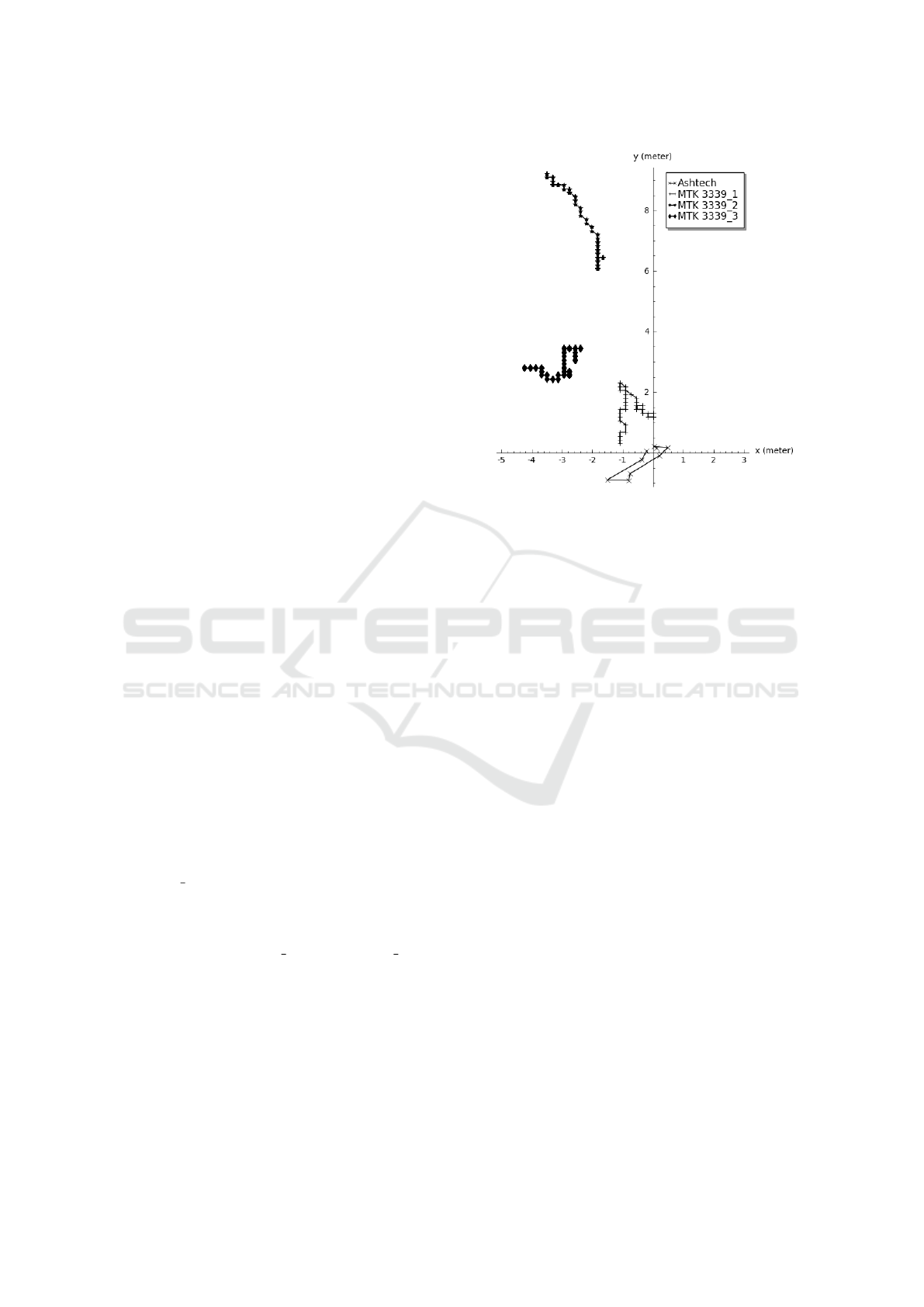
Figure 1 shows the results of a typical mea-
surement at the reference site. The origo of the
graph is the IGN reference coordinate for the site,
deviation from the origo means measurement error.
MTK3339 2 was not able to lock on the SBAS sig-
nal (even though the other two modules in its vicinity
were eventually able to receive SBAS corrections),
this fact is reflected in its much less precise mea-
surements than MTK3339 1 and MTK3339 3. The
two modules that did lock on SBAS produced much
less precise locations than the 1 meter error required.
Even the advanced Ashtech reference receiver had a
maximum error that was larger than 1 meter.
The maximum error relative to the reference point
measured with the MTK3339 was in the 2.22-11.51
meters range. All the measurements were made in
an environment that models agricultural conditions:
mostly flat area with minor depressions, low vegeta-
Figure 1: Results of one measurement at Ecouflant I site.
tion with occassional trees. The reference coordinates
were either taken from the Ashtech receiver (when
the measurement was not performed at the geodetic
reference point) or were the coordinates specified by
IGN for the reference point. The measurement ses-
sions lasted 10 minutes, measured from the moment
when all the 3 SBAS receivers locked on the SBAS
signal. This could take quite a long time depending
on the location and time of the day, it was quite com-
mon that 10-15 minutes needed from the first GPS
location fix to the first SBAS fix and there were mea-
surements when one module could not even obtain
SBAS fix, in spite of the fact that the SBAS receivers
were placed very near to each other (3 centimeters).
When the SBAS signal was not acquired, the maxi-
mum error was 30.89 meters. Our conclusion based
on the field measurements is that low-cost GPS re-
ceivers even with SBAS differential corrections are
not able to satisfy our requirement of 1 meter accu-
racy. In addition, SBAS signal cannot be reliably ac-
quired on ground level.
3 EVALUATION OF LOW-COST
DIFFERENTIAL GPS
Our measurements presented in section 2 convinced
us that a low-cost GPS receiver supporting only the
L1 band is only able to support our accuracy re-
quirements if it is used in differential mode. The
goGPS software (Herrera et al., 2016) was created
to support exactly these kinds of receivers with dif-
Cost-efficient Localisation System for Agricultural Use Cases
143
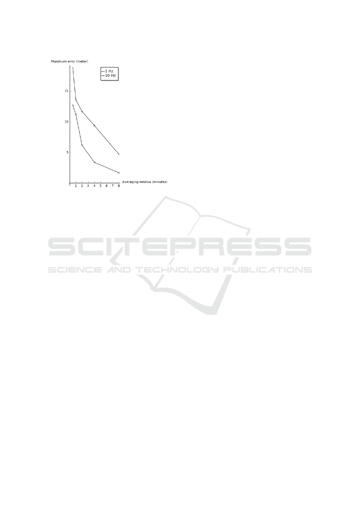
Figure 2: Maximum position error as a function of sampling
frequency and averaging time.
ferential support. Readers interested in the details
of goGPS should consult the cited references, only a
brief overview is presented here.
In order to enhance the baseline accuracy of low-
cost receivers, goGPS relies on raw observation data
(pseudorange, carrier phase) from the GPS receiver,
provided by the u-blox LEA-6T receiver in our case.
We used goGPS in off-line mode when the rover and
the master are not connected during the measure-
ments. It is possible to set up the system with two
low-cost receivers (one in master role located at a
well-known coordinate and one in rover role) or with
one professional reference station in master role (we
used IGN’s NGER reference station which is about 10
km from the location where the measurements were
made) and a low-cost receiver in rover mode.
Double differencing in differential GPS mode
eliminates efficiently the effect of ionospheric delay
but other error terms like random noise, multipath ef-
fects and receiver clock errors still affect the locations
calculated by the goGPS software. Figure 2 shows
the maximum position error when the GPS receiver
sampling frequency was 1 Hz and 10 Hz as a func-
tion of sliding averaging window length. The window
length was between 0.5 min and 8 min. The figure
demonstrates that the residual position error can be
efficiently decreased with low-pass filtering but this
affects the temporal sensitivity of the system which
cannot be compensated by increasing the receiver’s
sampling frequency.
The effect of high-quality reference station mas-
ter vs. using a low-cost receiver as master was also
evaluated. High-quality reference station decreases
the noise of at least the master receiver. On the other
hand, the IGN reference station had a sampling pe-
riod of 30 seconds. The goGPS software assumes a
1:1 relationship between rover and master samples,
discarding rover samples if there is no corresponding
master sample. The outcome is a significant reduc-
tion of effective sampling frequency which reduces
the averaging window size to achieve the same tem-
poral sensitivity. We evaluated the effect in two mea-
surements and we found that the maximum error with
low-cost master station was 1.3 meters while the max-
imum error with IGN master was 3.31 meters. While
this measurement cannot be considered extensive, it
indicates that high-quality master may improve the
accuracy only if its sampling frequency is compara-
ble with that of the rover.
We conclude that goGPS is indeed capable of pro-
ducing location measurements using data from low-
cost receivers if the target is stationary for at least 8-
10 minutes. In case of moving targets (in particular in
case of targets moving unpredictably like the cows)
its error quickly increases so that trajectory tracking
becomes impossible.
4 BEHAVIOURAL ANALYSIS OF
DAIRY COWS
In this section we analyse whether it is possible to
measure cow location in spite of the restriction im-
posed by goGPS’ deficiency in tracking moving tar-
gets. The other use case is simpler as we control the
movement of the robot entirely so if there is a need of
a precise location fix, we can stop the movement for
the required period. Cows, however, move according
to their will and if they do not stay stationary for long
enough, the low-cost rover will not be able to acquire
the target’s accurate position even occasionally. This
phase of the research was accomplished based on data
sets acquired by earlier research projects. (Wietrzyk
and Radenkovic, 2007) (from now called Notting-
ham measurement) tracked 6 dairy cows for 2 days
using GPS collars. Based on our experiences about
GPS accuracy (see section 2), we consider the target
stationary if its location does not change more than
3 meters from the baseline position acquired when
the assumed stationary period started for 10 minutes.
(De Weerd et al., 2015) (from now called Weerd mea-
surement) tracked 9 cows for 11 days and added hu-
man observations to high-frequency GPS data. Hu-
man observations attach 7 labels to high-frequency
GPS data of which we considered 5 (“Drinking”,“Dry
forage”,“Foraging”,“Standing”, “Grooming”) as sta-
tionary. If the animals stayed for at least 10 minutes
SENSORNETS 2017 - 6th International Conference on Sensor Networks
144

Figure 3: Stationary time per cow, Nottingham measure-
ment.
in a stationary state, then the time spent in the state
was added to the stationary time. The total stationary
time was derived in this case entirely from human-
observed labels. We processed only open-field (as op-
posed to forest) measurement in this paper.
Figure 3 presents the stationary time for the Not-
tingham measurement, by cow. One cow was found
to be stationary all the time and its data has been elim-
inated from this chart. In general, the cows spend 40-
90% of their time stationary even though the one with
ID of ”067” was constantly moving. Eventually on
average the 5 cows were stationary for 62.3% of their
time.
The Weerd measurement presented much more
uniform picture. All the 9 cows were found to be sta-
tionary between 79.5 %-89.8 % of the time with an
average of 80.9 %. We therefore concluded that even
though the movement pattern of the animals depends
on the particular cow, it can be assumed with high
probability that at least some animals in the group stay
stationary for the time period needed for an accurate
GPS measurement. These animals can be used as ref-
erence points to locate the animals that were found
to be moving with short-range distance or angle mea-
surement methods.
5 DISTANCE-BASED
SHORT-RANGE
LOCALISATION
The problem of the distance-based short-range lo-
calisation is the following. We intend to localise a
point with unknown position on a 2D map based on
distance measured from reference points with well-
known positions. We can then calculate the position
of the unknown point with a trilateration algorithm
(Cheung et al., 2006). We assume that the cows are
equipped with an Ultra-Wideband (UWB) range mea-
suring system and a GPS. There are competing UWB
technologies on the market that we are still evaluat-
ing. UWB system is for the relative distance estima-
tion among the animals and the GPS is for absolute
positions. We have to understand how the errors of
each system affect the unknown position’s estimation
error. Trilateration studies often omit the error to sim-
plify the equations’ resolution.
The first part of our simulation is a simple problem
with N well-known fixed points. If we measure all the
distances r
n wpt/u
between the well-known points with
the following coordinate [x
n wpt
,y
n wpt
] with n wpt =
1,...,N and the unknown point [x
u
,y
u
], we can find the
unique point, only if all the well-known points are not
aligned. a system with simple circles equations give
this results.
5.1 The Effect of Distance
Measurement Error
In the first simulation we tried to find how an error
on distance measurement could affect the reconstruc-
tion of the unknown point. The aim of this simu-
lation is to verify if we can reconstruct the position
of an unknown point and to determine what is the
error of the unknown point estimation in the pres-
ence of distance measurement error. We have tried
N = {4,5,6,10,20}. We chose the location of these
well-known points according to real grazing situa-
tion. In (Dumont et al., 2005), the domestic herbi-
vores used to graze in group. Few animals are alone.
The selected plot is an area of maximum 300 meters
× 300 meters. As example, this is the coordinate for
10 fixed points: [0,0] ; [0, 5] ; [−10,10] ; [−10,−6] ;
[100,100] ; [10,−8] ; [70,−40] ; [80,−45] ; [75,−35]
; [−5,90]. A random point is picked in the area. The
exact radius could be calculated with the knowledge
of the fixed points and random point coordinates. A
different random error of ε meters is added to each ra-
dius to reflect the error. Finally this overdetermined
system is described in the following equation:
(x
u
− x
1
)
2
+ (y
u
− y
1
)
2
− (
q
(x
1
− x
u
)
2
+ (y
1
− y
u
)
2
+ ε
1
)
2
= 0
.
.
.
(x
u
− x
N
)
2
+ (y
u
− y
N
)
2
−
(
q
(x
N
− x
u
)
2
+ (y
N
− y
u
)
2
+ ε
N
)
2
= 0
(1)
This system in this form is a non-linear least-squares
problem. We use iterative non-linear least-squares al-
gorithm to solve these equations due to distance mea-
Cost-efficient Localisation System for Agricultural Use Cases
145
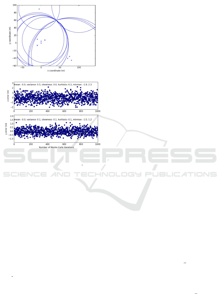
Figure 4: Optimal situation for 10 fixed points.
Figure 5: Example of the error repartition on x and y.
surement errors. In our simulation each ε
n wpt
is a ran-
dom value between ±2 meters. Using Python’s scipy
package, we iterate the process 1 000 times to act as a
Monte-Carlo test and we repeat the process with 100
random and unknown points. Figure 4 represents the
ideal situation with 10 well-known points. Figure 5
represents the error after 1 000 iterations for a given
list of well-known points.
The results are presented in table 1 with regards
to different number of fixed points. ∆
max
is the dif-
ference between the maximum error and the mini-
mum error for all the situations. So it is the upper
bound of the error for all the situations (and itera-
tions). ∆
mean(ε
b
X
u
)
represent the upper bound of the
mean of errors on one axis. max(σ
2
b
X
u
) is the maxi-
mum of the variance in all the situations. [
b
X
u
;
b
Y
u
] is a
N × 2 matrix size of all the estimation results of the
unknown point.
We have started the iterative algorithm
(least squares() from the scipy Python library)
from the same initial point and we experienced that
the results were slightly different after the end of
each iterative process. Therefore we executed the
iterative process several times and we took the mean
of the results. Our experience is that this mean value
is of better quality than any of the standalone results.
In the following simulations, however, we considered
that each distance measurement has a different
measurement error. We consider that we only have
one chance to calculate the unknown position to save
power in the real case.
The main problem of this simulation is to help
the algorithm to find the correct minimal solution.
Optimisation functions are very susceptible to initial
state. When the number of well-known points is not
enough, a good solution is hard to find. That why the
variances are very high for 4 and 5 fixed well-known
points. Moreover, in 4 and 5 fixed points, we try to
model a real grazing situation, so animals are really
close. A group of reference points that are close to
each other could behave as if they were one point.
This situation is not suitable to estimate the position
if no reference points are available that are far away
from this group. The reason of this phenomenon is the
small distance between the first points, the large dis-
tance to the last point, and the addition of a random
error.
In conclusion, our simulation shows it is impor-
tant to have at least 3 fixed points which are far away
to be sure of the good problem resolution. This result
is interesting to minimise the calculation load in an
embedded system and to help us to evaluate the num-
ber of UWB anchors. Moreover, if a group of cows
is close to each other, it is possible to activate only a
part of the GPS receivers in the group to save power.
5.2 Effect of Reference Point Position
Error
We consider using GPS to obtain the coordinates of
the fixed points and to use UWB to measure the dis-
tance between the fixed points and the unknown point.
In that case, the GPS error may introduce a more sig-
nificant error source. We made a second simulation
to understand the consequence of a GPS localisation
error in the reconstruction of the unknown point. In
this situation, we consider no distance measurement
error.
The aim is to reduce the system to linear equa-
tions. The new system can be written as:
(x
N
− x
1
) · x
u
+ (y
N
− y
1
) · y
u
=
1
2
(r
2
1
− r
2
N
+ x
2
N
− x
2
1
+ y
2
N
− y
2
1
)
.
.
.
(x
N
− x
N−1
) · x
u
+ (y
N
− y
N−1
) · y
u
=
1
2
(r
2
N−1
− r
2
N
+ x
2
N
− x
2
N−1
+ y
2
N
− y
2
N−1
))
(2)
SENSORNETS 2017 - 6th International Conference on Sensor Networks
146
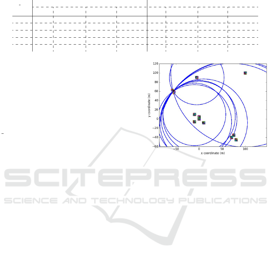
Table 1: Statistics on all the unknown point estimation in distance error situation in meter.
n wpt x (meter) y (meter)
pts ∆
max
mean(ε
b
X
u
) ∆
mean(ε
b
X
u
)
max(σ
2
b
X
u
) ∆
max
mean(ε
b
Y
u
) max(σ
2
b
Y
u
) ∆
mean(ε
b
Y
u
)
4 23.6 -0.1 39 2.4 24.6 0.1 43.9 2.4
5 24.32 -0.1 37.8 3.8 23.6 0.0 43.0 4.0
6 12.5 0.0 5.5 0.3 14.8 0.0 7.8 0.3
10 9.7 0.0 2.9 0.2 9.9 0.0 2.7 0.1
20 6.2 0.0 1.2 0.1 6.4 0.0 1.0 0.1
This could be put in a matrix form (equation 3).
Subtracting the last equation from the other equations
is arbitrary.
Gβ = F (3)
where G =
x
N
− x
1
y
N
− y
1
.
.
.
.
.
.
x
N
− x
N−1
y
N
− y
N−1
, β =
x
u
y
u
, F =
1
2
·
r
2
1
− r
2
N
+ x
2
N
− x
2
1
+ y
2
N
− y
2
1
.
.
.
r
2
N−1
− r
2
N
+ x
2
N
− x
2
N−1
+ y
2
N
− y
2
N−1
The localisation estimation could be found with this
linear equation using the standard linear least-squares
method (eq. 4).
b
β = (G
T
G)
−1
G
T
F (4)
b
β is the estimated coordinate.
To visualize the problem, the figure 6 represents
10 fixed points with 1 000 different simulated errors
added to them and the estimation of the unknown
point. One larger patch in this figure represents a ref-
erence point with a set of error values added.
The results of this simulation are presented in ta-
ble 2. For 10 fixed points in this configuration, the
results are good. In some cases with few fixed points,
this table show some variance problem. Sometime the
simple resolution does not work and the result of the
least-squares solution exhibits a large error. A low-
pass filter that we did not implement could be used to
control the problem.
The calculation takes approximately 20 to 50 sec-
onds with the linear least-square method and 520 sec-
onds to 715 seconds with the iterative non-linear al-
gorithm proportion to the number of fixed points de-
pending on the number of fixed points. The processor
used is an Intel i7-4700MQ, 2.4 GHz and the com-
puter is equipped with 16 GBytes of volatile memory.
We can conclude that linear least-square algorithm
could be used if we have enough separate fixed points.
If we have enough computation resources and not
enough separate fixed points, we could use non-linear
least-square techniques to find the correct unknown
Figure 6: Representation of 10 fixed points with simulated
error added to them and the effect of the error of the locali-
sation of the unknown point.
point. We can see that for a same measurement error,
in our case ±2 meters, with enough separated fixed
points, the estimation is better if we assume that the
measurement error is introduced into the fixed points’
positions. In our real study, the distance measurement
could be given by UWB which have, theoretically, a
better accuracy than ±2m. Finally the error position
could only depend on the effect of reference point po-
sition error. But we have to do other simulation and
try.
6 ANGLE-BASED SHORT-RANGE
LOCALISATION
Beside distance-based short-range localisation, we in-
vestigated whether we can build an in-house angle-of-
arrival (AOA) short range localization system. This
localisation method depends on a direction-sensitive
antenna. The antenna rotates and finds out the angle
of signals from stations with known locations. These
stations can either be fixed to the ground or mounted
to a moving platform which stops for long enough
time periods so that it can be localised accurately (see
section 3).
Our AOA localisation method is based on the prin-
Cost-efficient Localisation System for Agricultural Use Cases
147
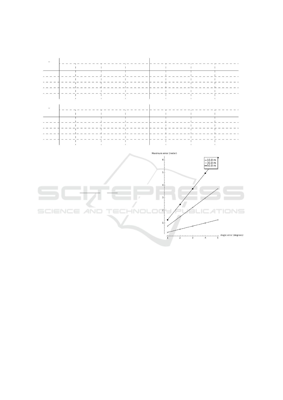
Table 2: Statistics on all the unknown point estimation in fixed points error situation in meters.
linear least-squares solution
n wpt x (meter) y (meter)
pts ∆
max
mean(ε
b
X
u
) ∆
mean(ε
b
X
u
)
max(σ
2
b
X
u
) ∆
max
mean(ε
b
Y
u
) ∆
mean(ε
b
Y
u
)
max(σ
2
b
Y
u
)
4 4·10
6
49.1 4341 15·10
9
4·10
6
-50.9 4473 16·10
9
5 128.3 0.0 1.7 223.6 134.6 0.0 1.9 269.1
6 19.7 0.0 0.3 9.6 18.4 0.0 0.5 10.5
10 19.9 0.0 0.4 10.0 20.0 0.0 0.5 12.6
20 12.7 0.0 0.4 5.0 12.3 0.0 0.3 5.6
non-linear least-squares solution
n wpt x (meter) y (meter)
pts ∆
max
mean(ε
b
X
u
) ∆
mean(ε
b
X
u
)
max(σ
2
b
X
u
) ∆
max
mean(ε
b
Y
u
) ∆
mean(ε
b
Y
u
)
max(σ
2
b
Y
u
)
4 338 -0.1 5.9 178 370 0.1 189
5 344.8 0.1 5.6 169.4 368.5 0.1 6.3 167.0
6 13.8 0.0 0.2 5.8 15.6 0.0 0.3 9.2
10 9.4 0.0 0.2 2.6 10.0 0.0 0.2 2.8
20 7.2 0.0 0.1 1.4 6.4 0.0 0.1 0.9
ciples described in (Cheung et al., 2006). We assume,
however, that instead of the fixed stations measuring
the angle of the mobile station’s beacon signal, it is
the mobile station that measures the angle of the fixed
stations’ beacon signal. So equation (47) in (Cheung
et al., 2006) changes to equation 5.
tan(r
AOA,i
) =
sin(r
AOA,i
)
cos(r
AOA,i
)
=
y
i
− y
x
i
− x
(5)
where r
AOA,i
is the angle of the ith fixed station as
measured by the mobile station, x
i
,y
i
is the known
position of the ith fixed station, and β =
x
u
y
u
is the
unknown position of the mobile station. By bringing
this set of equations to a linear matrix form, we get
H =
−sin(r
AOA,1
) cos(r
AOA,1
)
.
.
.
.
.
.
−sin(r
AOA,N
) cos(r
AOA,N
)
(6)
k =
−x
1
sin(r
AOA,1
) + y
1
cos(r
AOA,1
)
.
.
.
−x
M
sin(r
AOA,N
) + y
M
cos(r
AOA,N
)
(7)
where N is the number of the fixed stations whose
angle is measured. N is at least 3 but the measure-
ment may be overdetermined where N > 3 hence lin-
ear least-square solution is calculated.
ˆ
β = (H
T
H)
−1
H
T
k (8)
We have made simulations to estimate the localisation
accuracy. Figure 7 shows the localisation error mea-
sured in a simulation with varying angle measurement
error and distance between the mobile station and the
Figure 7: AOA localisation accuracy as a function of the
distance to the fixed stations and angle measurement error.
fixed stations. The 4 fixed stations were arranged in
a square, the mobile station was from equal distance
from all the fixed stations. The distance shown in the
figure is the distance between the mobile station and
any of the fixed stations. We assumed that there is a
fixed measurement error (x axis). The angle measure-
ment error was added to the exact angles so that the
distance between
ˆ
β and β is maximal and this maxi-
mum error is shown in the figure.
With the distance of 50 meters, the required lo-
calisation precision can be achieved only if the an-
gle measurement error is less than 1 degree. We
built a simple prototype to verify how easily these
requirements can be implemented based on Atmel
ATmega328P MCU (Arduino Pro Mini) and Nordic
nRF24L01P RF module, operating in the 2.4 GHz
SENSORNETS 2017 - 6th International Conference on Sensor Networks
148

band. The sender unit was equipped with a simple
omnidirectional stick antenna and the receiver unit
was equipped with a 9 dBm PCB Yagi antenna. By
turning around the Yagi antenna, the angle range (0
degree being the direction of the sender) was iden-
tified where the sender’s data can be received. Un-
fortunately the nRF24L01P module has no Received
Signal Strength Indicator (RSSI) feature, the signal is
either present or not. This means that there is a min-
imum distance to the sender because if the receiver
is closer to the sender than the minimal distance, the
signal can be received independently of the angle of
the receiver’s antenna. This restriction can be miti-
gated by a receiver that provides RSSI along with the
received data packets.
The measurements were made on an agricultural
field that serves as a pasture. The sender’s trans-
mission power was set to one of the 3 levels the
nRF24L01P supports. The receiver was located at
a specified distance from the sender and the antenna
was rotated. The angle when the signal appeared and
when the signal disappeared was recorded. With this
simple method the direction of the sender was iden-
tifiable with 1 degree precision. The minimum and
maximum distances with different power levels were
the following: PA MIN: 4-20 meters, PA LOW: 22-
41 meters, PA HIGH: 31-70 meters.
7 CONCLUSIONS
Low-cost, accurate localisation is often required in
agricultural applications. We found that low-cost GPS
modules are inadequate but in differential setup cer-
tain low-cost modules are able to produce the required
accuracy if the target is stationary for at least 8-10
minutes. Certain cows (but not all of them) were
found to satisfy the criteria for being stationary for
40-80 % of their grazing time. Movements have to
be tracked by an auxiliary technology. We made sim-
ulations for two of such technologies: distance- and
angle-based short-range localisation technology. In
case of distance-based, the effect of distance mea-
surement error results in worse position estimation
than the effect of reference point measurement error.
Angle-based short-range localisation turned out to be
more cost-efficient but also more problematic, due to
the rapidly growing localisation error as the distance
between the mobile and the fixed station grows.
ACKNOWLEDGEMENTS
The Hungarian side of the research is supported by
the AgroDat.hu project (project code: VKSZ 12-1-
2013-0024), financed by the Government of Hungary.
I thank ESEO for co-financing my research stay in
Angers, France where part of the research was done.
The French side of the research is financed by the re-
gion of ”Pays de la Loire” (Vagabond project).
REFERENCES
Cheung, K. W., So, H. C., Ma, W.-K., and Chan,
Y. T. (2006). A constrained least squares approach
to mobile positioning: Algorithms and optimality.
EURASIP J. Appl. Signal Process., 2006:150–150.
De Weerd, N., van Langevelde F., and van Oeveren H.,
e. a. (2015). Deriving animal behaviour from high-
frequency gps: Tracking cows in open and forested
habitat. PLoS ONE. 2015;10(6):e0129030.
Dumont, B., Boissy, A., Achard, C., Sibbald, A., and Er-
hard, H. (2005). Consistency of animal order in spon-
taneous group movements allows the measurement of
leadership in a group of grazing heifers. Applied Ani-
mal Behaviour Science, 95(1–2):55–66.
Herrera, A. M., Suhandri, H. F., Realini, E., Reguzzoni, M.,
and Lacy, M. C. (2016). goGPS: Open-source MAT-
LAB software. GPS Solut., 20(3):595–603.
Langley, R. B. (1991). The mathematics of gps. GPS World,
pages 45 – 50.
Paller, G. and
´
El
˝
o, G. (2016). Power consumption con-
siderations of an agricultural camera sensor with
image processing capability. In 2nd International
Conference on Sensors and Electronic Instrumen-
tal Advances (SEIA’ 2016), 22-23 September 2016,
Barcelona, Castelldefels, Spain.
Wietrzyk, B. and Radenkovic, M. (2007). CRAWDAD
dataset nottingham/cattle (v. 2007-12-20). Down-
loaded from http://crawdad.org/nottingham/cattle/
20071220.
Cost-efficient Localisation System for Agricultural Use Cases
149
