Quantum-enhanced Metrology without Entanglement

based on Optical Cavities with Feedback

Lewis A. Clark, Adam Stokes, M. Mubashir Khan, Gangcheng Wang and Almut Beige

The School of Physics and Astronomy, University of Leeds, Leeds LS2 9JT, U.K.

Keywords:

Quantum Metrology, Optical Cavities, Quantum Feedback.

Abstract:

There are a number of different strategies to measure the phase shift between two pathways of light more

efﬁciently than suggested by the standard quantum limit. One way is to use highly entangled photons. Another

way is to expose photons to a non-linear or interacting Hamiltonian. This paper emphasises that the conditional

dynamics of open quantum systems provides an interesting additional tool for quantum-enhanced metrology.

As a concrete example, we review a recent scheme which exploits the conditional dynamics of a laser-driven

optical cavity with spontaneous photon emission inside a quantum feedback loop. Deducing information from

second-order photon correlation measurements requires neither optical non-linearities nor entangled photons

and should therefore be of immediate practical interest.

1 INTRODUCTION

This paper compares different strategies to decrease

the uncertainty ∆ϕ for measurements of an unknown

phase shift ϕ between two pathways of light when

given a certain amount of resources N. Using N in-

dependent resources, i.e. deducing ϕ from a measure-

ment signal M(ϕ) obtained from the dynamics of a

generator which is linear in N, the scaling of the lower

bound of the uncertainty ∆ϕ of the phase measure-

ment with respect to N is given by the standard quan-

tum limit (Dowling and Seshadreesan, 2015),

∆ϕ

class

∝ N

−0.5

. (1)

However, using for example N highly-entangled pho-

tons as a resource, the measurement uncertainty ∆ϕ

can be as low as the Heisenberg limit,

∆ϕ

quant

∝ N

−1

. (2)

An alternative way of enhancing metrology beyond

the standard quantum limit is to expose N incoming

single photons to a ϕ-dependent Hamiltonian which

is no longer linear in N (Boixo et al., 2008). In this

case, the uncertainty ∆ϕ of the phase measurement

scales as

∆ϕ

non−lin

∝ N

−0.5k

, (3)

where k denotes the order of non-linearity of the

interaction Hamiltonian with respect to N or de-

scribes the interaction between k phase dependent

systems. However, multi-photon entanglement and

highly-efﬁcient optical non-linearities are hard to im-

plement experimentally and have not yet become

readily available for a wide range of applications.

Some suggested schemes avoiding entanglement to

get an enhancement include the use of non-linear op-

tics (Luis, 2007) or using squeezed states (Caves,

1981).

In some situations, the length of the measurement

process, t, and not the number of incoming photons,

N, is the main resource which we want to constrain

(Clark et al., 2016b). If we can write the time t in

such cases as t = N ∆t with ∆t being the length of a

short time interval, then the standard quantum limit

still coincides with Eq. (1). In the following we em-

phasise that the environmental interactions of open

quantum systems naturally result in conditional dy-

namics, like quantum jumps (Blatt and Zoller, 1988),

which can be exploited for quantum computational

tasks (Beige et al., 2000; Lim et al., 2005; Metz et al.,

2006; Clark et al., 2015). It is shown that the gen-

erators of the conditional dynamics can introduce a

non-linear resource-dependence with respect to time

(Clark et al., 2016c). Applying this observation to

quantum metrology provides an additional tool which

allows us to break the standard quantum limit (1) and

helps us to design scheme which can be implemented

relatively easily.

As an example, we review a recent quantum-

enhanced metrology scheme by Clark et al. (Clark

et al., 2016b) which requires only a laser-driven op-

tical cavity inside a quantum-feedback loop. The pro-

posed setup is feasible with current technology (Kuhn

A. Clark L., Stokes A., Mubashir Khan M., Wang G. and Beige A.

Quantum-enhanced Metrology without Entanglement based on Optical Cavities with Feedback.

DOI: 10.5220/0006141702230229

In Proceedings of the 5th International Conference on Photonics, Optics and Laser Technology (PHOTOPTICS 2017), pages 223-229

ISBN: 978-989-758-223-3

223

et al., 2002; McKeever et al., 2004). Differing from

Ref. (Clark et al., 2016b), this paper does not pay as

much attention to the concrete analysis of the pro-

posed scheme. Instead, it focusses its attention on

what we believe to be the main mechanisms under-

lying the observed enhancement. Our ﬁndings com-

plement the work of other authors (Braun and Martin,

2011; Macieszczak et al., 2016; Pearce et al., 2015),

who also observe that quantum-enhancements may

be obtained from quantum correlations and sequential

measurements in open quantum systems.

There are ﬁve sections in this paper. Section 2 re-

views the main theoretical models that are commonly

used to describe quantum optical systems with spon-

taneous photon emission. In Section 3, we discuss

how to use the non-linear conditional dynamics of

an open quantum system to measure the phase shift

ϕ between two pathways of light, using the work of

Ref. (Clark et al., 2016b) as an example. Section 4

emphasises that the observed quantum enhancement

is not unexpected by showing that subsequent mea-

surements on a single quantum system provide at least

as much information as single-shot measurements on

entangled states. Finally, we summarise our ﬁndings

in Section 5.

2 THE QUANTUM JUMP

DYNAMICS OF OPEN

QUANTUM SYSTEMS

In this section, we review the modelling of open

quantum systems with spontaneous photon emission

(Hegerfeldt, 1993; Dalibard et al., 1992; Carmicheal,

1993; Stokes et al., 2012), thereby emphasising that

the conditional dynamics of single quantum trajecto-

ries, which is associated with quantum jumps, is nat-

urally non-linear.

2.1 The Schr

odinger Equation of

Closed Quantum Systems

As is well known, the dynamics of a closed quan-

tum system in the Schr

odinger picture is given by the

Schr

odinger equation,

ψi = −

H |ψi, (4)

where |ψi is a state vector and H is the time-

independent Hamiltonian and energy observable.

Solving the above equation for a given initial state

|ψ(0)i yields the state vector |ψ(t)i,

|ψ(t)i = exp



−



|ψ(0)i. (5)

This shows that the generator for the dynamics of a

closed quantum system is linear in time.

Suppose the Hamiltonian H depends on an un-

known parameter ϕ which we want to measures as

accurately as possible. Then the above closed system

dynamics, i.e. the time evolution of a measurement

signal M(t,ϕ), can be used to deduce ϕ. The longer

the system is observed and the larger the measure-

ment time t, the more information about ϕ becomes

available and the smaller the uncertainty ∆ϕ of this

measurement can become. However ∆ϕ is limited by

the standard quantum limit (1) with respect to the re-

source N which measures time.

2.2 Master Equations of Open

Quantum Systems

When interacting with an environment, the expecta-

tion values of physical observables averaged over an

ensemble of quantum systems can no longer be de-

duced from a single state vector |ψi. The ensem-

ble now needs to be described by a density matrix ρ.

For Markovian systems, ρ necessarily obeys a master

equation of Lindblad form. For example, the mas-

ter equation of an open quantum system with sponta-

neous photon emission and only a single decay chan-

nel can be written as (Stokes et al., 2012)

ρ = L ρ (6)

with the linear superoperator L given by

L ρ = −

[H,ρ] +



2LρL

†

−

†

L,ρ



(7)

Here Γ denotes the spontaneous decay rate and L is

the so-called Lindblad operator. In the case of an op-

tical cavity, L simply coincides with the cavity pho-

ton annihilation operator c and Γ becomes the spon-

taneous cavity decay rate κ. In analogy to Eq. (5) we

now ﬁnd that

ρ(t) = exp (Lt) ρ(0), (8)

where ρ(0) denotes the initial state of the open quan-

tum system. As in the previous subsection, we see

that the generator of the system dynamics is linear in

time. This is analogously to the situation of closed

quantum systems in the previous subsection. The

standard quantum limit (1) still gives a lower bound

for the uncertainty ∆ϕ for the measurement of an un-

known parameter ϕ with respect to time.

2.3 Unravelling into Quantum

Trajectories

Having a closer look at microscopic derivations of

Eq. (6) (see e.g. Refs. (Hegerfeldt, 1993; Dalibard

PHOTOPTICS 2017 - 5th International Conference on Photonics, Optics and Laser Technology

224

et al., 1992; Carmicheal, 1993; Stokes et al., 2012))

shows that Eq. (6) is the result of averaging over

all possible quantum trajectories that the quantum

system can experience. If the system is continu-

ously monitored and all its photon emission times are

known, then it can still be described by a pure state

vector at all times. To point out the relevant unravel-

ling of Eq. (6), we now write the derivative

ρ as

ρ = −

cond

ρ −ρH

†

cond

+ ΓLρL

†

(9)

with H

cond

being the non-Hermitian conditional

Hamiltonian given by

cond

= H −

~ΓL

†

L (10)

and with L being the same Lindblad operator as in

Eq. (7). Re-writing our master equation in this com-

pact form allows us to identify two subensembles.

The ﬁrst term in Eq. (9) is the time derivative of

the unnormalised density matrix of the subensemble

of quantum systems without a photon emission in a

small time interval (t,t + ∆t), while the second term

refers to the subensemble experiencing an emission.

The normalisation of both terms indicates their rela-

tive sizes.

More concretely, under the condition of no photon

emission in (t,t + ∆t), the state vector |ψ(t)i evolves

such that

|ψ(t + ∆t)i = K

|ψ(t)i/kK

|ψ(t)ik (11)

with the operator K

being the conditional no-photon

time evolution operator

= exp



−

cond

∆t



. (12)

The generator of the no-photon time evolution of our

open quantum system is again linear in time. How-

ever, in case of a photon detection in (t,t + ∆t), the

state vector of the quantum system changes into

|ψ(t + ∆t)i = K

|ψ(t)i/kK

|ψ(t)ik (13)

with the reset operator K

given by

= (Γ∆t)

1/2

L . (14)

In the case of a photon emission, a so-called quan-

tum jump occurs accompanied by sudden jumps of

expectation values (Blatt and Zoller, 1988). The gen-

erators of the conditional dynamics of open quantum

systems, which are associated with spontaneous pho-

ton emission, are in general highly non-linear due to

the constant need for resetting upon emission.

3 TEMPORAL QUANTUM

CORRELATIONS FOR

QUANTUM METROLOGY

Section 1 emphasises that generators of dynamics,

which are non-linear in the relevant resource, can be

used to measure an unknown parameter ϕ with an ac-

curacy ∆ϕ beyond the standard quantum limit. Sec-

tion 2 shows that the generators for the dynamics

of the single quantum trajectories of open quantum

systems are in general non-linear. Combining these

two observations, one can design novel quantum-

enhanced metrology schemes which require neither

entanglement nor a non-linear or interacting Hamil-

tonian. To illustrate this fact we now review a recent

proposal by Clark et al. (Clark et al., 2016b) based

on a single optical cavity inside a quantum feedback

loop for which time is the resource which we want to

constrain.

3.1 A Quantum-enhanced Metrology

Scheme

The quantum metrology scheme in Ref. (Clark et al.,

2016b) consists of two main stages, a preparation and

a measurement stage. These implement the following

tasks:

1. Firstly, the preparation stage prepares the cavity

ﬁeld in a coherent state |αi with α being of the

form

α = |α|e

iϕ

. (15)

One way of achieving this is to drive the cav-

ity with a laser ﬁeld that experiences the phase

shift ϕ and to let it relax into its stationary state

(c.f. Fig. 1).

2. Afterwards, during the measurement stage, the

cavity is placed inside a quantum feedback loop

(c.f. Fig. 2). Whenever a spontaneously emitted

photon is detected, a laser pulse is applied. This

laser pulse displaces the coherent state inside the

resonator in a certain direction, which should be

independent of ϕ. For simplicity, we assume here

that the feedback pulse is approximately instanta-

neous.

Since the feedback laser does not experience the un-

known phase ϕ, it provides a reference frame. What

the proposed metrology scheme measures is the rel-

ative phase between the laser ﬁeld applied during the

preparation stage and the quantum feedback laser. Al-

ternatively we could choose the preparation laser as

the reference frame, since this would not change the

Quantum-enhanced Metrology without Entanglement based on Optical Cavities with Feedback

225

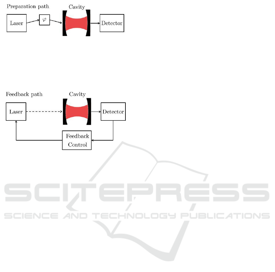
Figure 1: Schematic view of the preparation stage. Its pur-

pose is the preparation of the coherent state |αi given in

Eq. (15), which depends on the unknown phase shift ϕ. One

way of achieving this is to drive a leaky optical cavity with

a laser ﬁeld which experiences ϕ until the system reaches

its stationary state.

Figure 2: Schematic view of the measurement stage. Dur-

ing this stage, the cavity is placed inside a quantum feed-

back loop. The detection of photon emissions now triggers

a laser pulse that displaces the resonator ﬁeld in a certain

direction. The relative phase between the laser ﬁeld ap-

plied during the preparation stage and the quantum feed-

back laser can be deduced, for example, from second-order

photon correlation measurements with an accuracy that in-

creases rapidly in time.

dynamics of the system. Although doing so might be

less favourable in practical applications, let us assume

for the rest of the paper that this is the case for the sake

of convenience.

In standard approaches to quantum metrology

(Dowling and Seshadreesan, 2015; Giovannetti et al.,

2006), the relevant resource is the number of photons

experiencing the unknown phase shift ϕ. This is due

in part to the nature of interferometric experiments.

Usually N photons are passed through an interferom-

eter that contains the unknown phase before being

measured at the end. In the following we extract ϕ

from the photon statistics of the optical resonator dur-

ing the measurement stage. Hence in our scheme the

main resource is not the number of photons N pass-

ing through the setup but the number of observations

posed to deduce the photon statistics. This number is

directly proportional to the duration of the measure-

ment stage t which we can write as t = N ∆t.

3.2 The Non-linear Conditional

Dynamics of an Optical Cavity with

Feedback

As we have seen in Section 2, the expectation values

of an open quantum system with spontaneous pho-

ton emission averaged over all possible quantum tra-

jectories behave as if they were generated by linear

operators. However, to enhance quantum metrology

beyond the standard quantum limit without using en-

tanglement, we require our setup to behave as if its

dynamics were generated non-linearly. One way of

achieving this is to deduce the unknown parameter ϕ

from a measurement signal M(t,ϕ) corresponding to

a pre-selected subset of quantum trajectories, which

involves quantum jumps. In the following we there-

fore have a closer look at the dynamics of subsets

of quantum trajectories of the experimental setup in

Fig. 2.

For an optical cavity with spontaneous photon

emission the Lindblad operator is L = c, where c is

the usual bosonic photon annihilation operator. This

leads to a peculiar effect. If prepared in a coherent

state |αi, as it is in general the case for a laser-driven

optical cavity (Clark et al., 2016b), the spontaneous

emission of a photon does not change the ﬁeld inside

the resonator. In other words, there are no quantum

jumps in this case. The reason for this is that the co-

herent states are the eigenstates of the photon annihi-

lation operator c. To use the setup in Fig. 1 neverthe-

less for quantum-enhanced metrology, we either need

to prepare the cavity ﬁeld in a non-coherent state or

we need to replace L by another Lindblad operator.

A straightforward way of changing L is to intro-

duce quantum feedback. This is why we propose to

place the cavity during the measurement stage into a

quantum feedback loop, as illustrated in Fig. 2. If

the feedback operation depends on the unknown pa-

rameter ϕ, then its introduction moreover results in an

effective ϕ-dependence of the jump operation. More-

over, changing the state of the cavity upon the detec-

tion of photon essentially generates temporal corre-

lations in the conditional dynamics of the quantum

system. These correlations mean that the informa-

tion corresponding to an individual quantum trajec-

tory with respect to two or more different time steps

is no longer additive, thereby allowing for scaling be-

yond the standard quantum limit.

Taking quantum feedback into account in the the-

oretical model, which we introduced in Section 2, is

straightforward. The no-photon time evolution re-

mains the same. However, the operator K

in Eq. (14)

now needs to be replaced by R(ϕ)K

where R(ϕ) is

a unitary operator (Clark et al., 2016b; Clark et al.,

PHOTOPTICS 2017 - 5th International Conference on Photonics, Optics and Laser Technology

226

2015; Wiseman and Milburn, 2010). In other words,

all we have to do is to replace the Lindblad operator

L by another operator L(ϕ),

L −→ L(ϕ) = R(ϕ)L . (16)

For example, suppose every feedback operation R(ϕ)

displaces the coherent state inside the resonator by a

certain amount β(ϕ) such that

R(ϕ)|αi = |α + β(ϕ)i. (17)

Then the detection of a photon results indeed in an

effective quantum jump. An effective non-linearity

has been created which can be explored for quantum

metrology.

Breaking the standard quantum limit in Eq. (1)

when time is the resource which we want to constrain

requires that the dynamics of the cavity is very sensi-

tive to changes of the unknown parameter ϕ. In order

to be able to distinguish two parameters ϕ

and ϕ

the corresponding measurement signals M(t,ϕ

) and

M(t,ϕ

) need to evolve such that their distance grows

non-linearly in time. That this can be the case for the

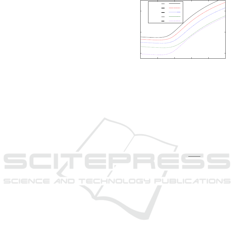
experimental setup which we consider here is illus-

trated in Fig. 3. Suppose β = |α(0)|e

iϕ

and ϕ = π.

Then the detection of a photon at t = 0 prepares the

cavity in its vacuum state, i.e. in the coherent state |αi

with α = 0. Fig. 3 is a logarithmic plot of |α(t)| aver-

aged over all quantum trajectories with a photon de-

tection during the ﬁrst time step of the measurement

stage (0,∆t) for different values ϕ which are all close

to π. All curves separate very quickly from the curve

corresponding to ϕ = π. Since the plot is logarithmic,

we see clearly that this happens in a highly non-linear

fashion with respect to time.

3.3 Second Order Photon Correlation

Functions

In order to obtain information about ϕ more efﬁ-

ciently than suggested by the standard quantum limit,

we need to ﬁnd a measurement signal M(t,ϕ), which

cannot be written as an ensemble average but depends

strongly on the appearance of quantum jumps. Taking

the discussion in the previous subsection into account,

we now have a closer look at the second-order photon

correlation function G

(2)

(t,t

), which is given by the

joint probability

(2)

(t,t

) ≡ I(t|t

)I(t

), (18)

where I(t|t

) denotes the probability for the detection

of a photon at a time t conditional on the detection of

a photon at t

. Second-order correlation functions are

usually normalised by the product of the photon emis-

sion rate at t

and at t. Doing so and dividing Eq. (18)

-2

0 0.2 0.4 0.6 0.8 1

Log (|α(t)|)



units of κ

−1



ϕ = π +

5π

ϕ = π +

4π

ϕ = π +

3π

ϕ = π +

2π

ϕ = π +

Figure 3: Logarithmic plot of |α(t)| averaged over all the

possible quantum trajectories of the subensemsbles with a

photon detection and a subsequently applies feedback op-

eration R(ϕ) during the ﬁrst time step of the measurement

stage (0,∆t) for ﬁve different values ϕ which are all close to

π. The ﬁgure is the result of a numerical simulation, which

averaged over 10

randomly generated quantum trajecto-

ries. Here we assume α(0) = 2 and β = |α(0)|e

iϕ

. More-

over, each time step ∆t is much smaller than the cavity pho-

ton life time 1/κ.

by I(t

)I(t), we deﬁne the renormalised second order

photon correlation function, g

(2)

(t,t

), by

(2)

(t,t

) ≡

I(t|t

)

I(t)

. (19)

Now g

(2)

(t,t

) depends no longer on the efﬁciency of

the detector shown in Fig. 2 and can be measured ac-

curately and relatively easily, even when using imper-

fect single-photon detectors.

Ref. (Clark et al., 2016b) uses measurements

of the second order photon correlation function

(2)

(t, 0), where t = N ∆t denotes the length of the

measurement stage, to deduce information about an

unknown phase ϕ between two pathways of light.

This means, we propose to measure the joint proba-

bility of detecting a photon at the start of the mea-

surement stage and another photon at the end, after a

time t. For simplicity, we ignore photon emissions be-

tween these two points. Nevertheless, we found that

the uncertainty ∆ϕ scales as N

−0.71

∆ϕ ∝ N

−0.71

, (20)

when ϕ = π and β = |α|, which surpasses the stan-

dard quantum limit (Clark et al., 2016b). Although

no entanglement is used, the origin of the quantum

enhancement in Eq. (20) is still of a quantum nature.

The second-order correlation function has no classi-

cal analogue and its measurement requires the detec-

tion of individual photons, although unit detection ef-

ﬁciency is not required.

What might seem most surprising about Eq. (20)

is that the measurement uncertainty ∆ϕ decreases

Quantum-enhanced Metrology without Entanglement based on Optical Cavities with Feedback

227

rapidly, as t increases. The longer one waits, the

more information is unvealed about ϕ. This again is

due to an interesting property of optical cavities in-

side instantaneous quantum feedback loops. A more

detailed analysis of the dynamics of the experimental

setup in Fig. 2 shows that the ﬁeld inside the resonator

never reaches a stationary state (Clark et al., 2016b;

Clark et al., 2016a) unless when being placed exactly

into its vacuum state. Whenever a photon is emit-

ted, a quantum feedback pulse occurs and increases

the number of photons inside the resonator. This in-

creases the probability for another photon emission

and so on. If the quantum feedback loop is truly

instantaneous, the mean number of photons inside

the cavity may easily diverge. Hence the longer one

waits, the more easily it becomes to distinguish these

two scenarios and to determine whether the system is

initially in its vacuum state or not. Here this question

is equivalent to asking whether ϕ = π or not.

Indeed the quantum enhanced-metrology scheme

in Ref. (Clark et al., 2016b) exploits the fact that

the cavity possesses two different types of dynam-

ics which separate in time. Similar effects have been

studied for example in Ref. (Macieszczak et al., 2016)

for quantum metrology applications. Due to the ef-

fective inﬁnite dimensional Hilbert space of the ﬁeld

inside an optical cavity, the divergence between both

types of dynamics may become arbitrarily large in

principle, thereby allowing for the scaling in Eq. (20)

to be preserved for an indeﬁnite time, which is not the

case for the scenarios studied in Ref. (Macieszczak

et al., 2016).

4 TEMPORAL QUANTUM

CORRELATIONS AND

ENTANGLEMENT

Suppose subsequent generalised measurements are

performed on a two-dimensional quantum system

prepared in |ψi. Moreover we assume that these mea-

surements can be described by two Kraus operators

and K

of the form

= |

ihξ

|, (21)

where |ξ

i and |ξ

i are two orthogonal states. How-

ever, no such constraint applies to |

i and |

In case of two measurements, the quantum system

changes such that

|ψi →











|ψi →



|ψi

|ψi →



|ψi

(22)

up to normalisation factors. Moreover, suppose we

perform a single-shot measurement of K

and K

two quantum systems prepared in an effective state

|ψ

eff

|ψ

eff

i =

√

|ξ

√

|ξ

√

|ξ

√

|ξ

i (23)

with the coefﬁcients p

i j

equal to

i j

= kK

|ψik

. (24)

One can easily see that both measurements yield the

outcome “i j” with exactly the same probability. The

state |ψi and |ψ

eff

i have the same information con-

tent. However, |ψ

eff

i is in general an entangled state.

For example, if K

= |ξ

ihξ

| and K

= |ξ

ihξ

|, we

ﬁnd that

|ψ

eff

i =

√

|ξ

√

|ξ

i. (25)

Analogously, one can show that N successive mea-

surements on a single system are in general equivalent

to a single-shot measurement of N entangled quantum

systems.

The quantum-enhanced metrology scheme that we

propose in Ref. (Clark et al., 2016b) extracts informa-

tion about the unknown phase ϕ between two path-

ways of light by performing N successive measure-

ments on a single quantum system. This means, our

scheme is equivalent to performing single-shot mea-

surements on a combination of N entangled quantum

systems. It is therefore not surprising that our scheme

can be used to break the standard quantum limit, as

the system possesses correlations. These are corre-

lations between the system and its environment. It

is the measurements upon the environment, i.e. the

measurement of photon emission, that accesses these

correlations.

5 CONCLUSIONS

This paper emphasises that the environmental inter-

actions of open quantum systems with spontaneous

photon emission naturally result in non-linear con-

ditional dynamics which can be exploited for quan-

tum metrology and other applications. More con-

cretely, we propose to deduce an unknown parame-

ter ϕ by measuring an expectation value M(t, ϕ) av-

eraged over a subset of preselected quantum trajec-

tories instead of measuring ensemble averages. If

the signal M(t, ϕ) evolves with a non-linear genera-

tor, the accuracy of the measurement ∆ϕ can exceed

the scaling proposed by the standard quantum limit

(Clark et al., 2016c). As an example, we reviewed

a recent quantum-enhanced metrology scheme which

PHOTOPTICS 2017 - 5th International Conference on Photonics, Optics and Laser Technology

228

measures the phase shift between two pathways of

light using the open system dynamics of the elec-

tromagnetic ﬁeld of an optical cavity inside a quan-

tum feedback loop (Clark et al., 2016b). This scheme

should be of immediate practical interest, since it re-

quires neither efﬁcient optical non-linearities nor en-

tangled photons.

ACKNOWLEDGEMENTS

AS and AB acknowledge ﬁnancial support from

the UK EPSRC-funded Oxford Quantum Technology

Hub for Networked Quantum Information Technolo-

gies NQIT. MMK acknowledges a postdoctoral re-

search fellowship funding from the Higher Education

Commission of the Government of Pakistan. GW ac-

knowledges ﬁnancial support from the NSF of China

(Grant No. 11405026) and Government of China

through a CSC (Grant No. 201506625070 ).

REFERENCES

Beige, A., Braun, D., Tregenna, B., and Knight, P. L.

(2000). Quantum computing using dissipation to re-

main in a decoherence-free subspace. Phys. Rev. Lett.,

85:1762.

Blatt, R. and Zoller, P. (1988). Quantum jumps in atomic

systems. Eur. J. Phys., 9:250.

Boixo, S., Datta, A., Flammia, S. T., Shaji, A., Bagan, E.,

and Caves, C. M. (2008). Quantum-limited metrology

with product states. Phys. Rev. A, 77:012317.

Braun, D. and Martin, J. (2011). Heisenberg-limited sensi-

tivity with decoherence-enhanced measurements. Nat.

Commun., 2:223.

Carmicheal, H. (1993). An Open systems Approach

to Quantum Optics, Lecture Notes in Physics, vol-

ume 18. Springer-Verlag, Berlin.

Caves, C. M. (1981). Quantum-mechanical noise in an in-

terferometer. Phys. Rev. D, 23:1693.

Clark, L. A., Huang, W., Barlow, T. M., and Beige, A.

(2015). Hidden Quantum Markov Models and Open

Quantum Systems with Instantaneous Feedback, vol-

ume 14, page 143. Springer International Publishing

Switzerland.

Clark, L. A., Maybee, B., Torzewska, F., and Beige, A.

(2016a). Non-ergodiciity and non-classical correla-

tions through quantum feedback. arXiv: 1611.03716.

(submitted).

Clark, L. A., Stokes, A., and Beige, A. (2016b). Quantum-

enhanced metrology through the single mode coher-

ent states of optical cavities with quantum feedback.

Phys. Rev. A, 94:023840.

Clark, L. A., Stokes, A., Khan, M. M., and Beige, A.

(2016c). Quantum jump metrology. to be submitted.

Dalibard, J., Castin, Y., and Mølmer, K. (1992). Wave-

function approach to dissipative processes in quantum

optics. Phys. Rev. Lett., 68:580.

Dowling, J. P. and Seshadreesan, K. P. (2015). Quan-

tum Optical Technologies for Metrology, Sensing, and

Imaging. J. Lightwave Technol., 33:2359.

Giovannetti, V., Lloyd, S., and Maccone, L. (2006). Quan-

tum metrology. Phys. Rev. Lett., 96:010401.

Hegerfeldt, G. C. (1993). How to reset an atom after a pho-

ton detection. Applications to photon counting pro-

cesses. Phys. Rev. A, 47:449.

Kuhn, A., Hennrich, M., and Rempe, G. (2002). Deter-

ministic single-photon source for distributed quantum

networking. Phys. Rev. Lett., 89:067901.

Lim, Y. L., Beige, A., and Kwek, L. C. (2005). Repeat-

until-success linear optics distributed quantum com-

puting. Phys. Rev. Lett., 95:030505.

Luis, A. (2007). Quantum limits, nonseparable transforma-

tions, and nonlinear optics. Phys. Rev. A, 76:035801.

Macieszczak, K., Guta, M., Lesanovsky, I., and Garrahan,

J. P. (2016). Dynamical phase transitions as a re-

source for quantum enhanced metrology. Phys. Rev.

A, 93:022103.

McKeever, J., Boca, A., Boozer, A. D., Miller, R., Buck,

J. R., Kuzmich, A., and Kimble, H. J. (2004). De-

terministic Generation of Single Photons from One

Atom Trapped in a Cavity. Science, 303:1992.

Metz, J., Trupke, M., and Beige, A. (2006). Robust entan-

glement through macroscopic quantum jumps. Phys.

Rev. Lett., 97:040503.

Pearce, M. E., Mehringer, T., von Zanthier, J., and Kok, P.

(2015). Precision Estimation of Source Dimensions

from Higher-Order Intensity Correlations. Phys. Rev.

A, 92:043831.

Stokes, A., Kurcz, A., Spiller, T. P., and Beige, A. (2012).

Extending the validity range of quantum optical mas-

ter equations. Phys. Rev. A, 85:053805.

Wiseman, H. M. and Milburn, G. J. (2010). Quantum Mea-

surement and Control. Cambridge University Press.

Quantum-enhanced Metrology without Entanglement based on Optical Cavities with Feedback

229