
Automatic Visual Detection of Incorrect Endoscope Adaptions in
Chemical Disinfection Devices
Timo Brune
1
, Björn Brune
2
, Sascha Eschborn
2
and Klaus Brinker
1
1
University of Applied Sciences Hamm Lippstadt, Marker Allee 76-78, Hamm, Germany
2
Olympus Surgical Technologies Europe, Kuehnstraße 61, Hamburg, Germany
Keywords: Computer Vision, Feature Detection, Surf, Sift, Registration, Machine Learning, Supervised Learning,
Endoscopes, Disinfection.
Abstract: This paper presents a complete analyzing system for detecting incorrect endoscope adaptions prior to the
use of chemical disinfection devices to guarantee hygienic standards and to save resources. The adaptions
are detected visually with the help of an image registration algorithm based on feature detection algorithms.
On top of the processing pipeline, we implemented a k-nearest neighbor algorithm to predict the status of
the adaption. The proposed approach shows good results in detecting the adaptions correctly.
1 INTRODUCTION
Endoscopic diagnostic is the main application for
diseases of the gastrointestinal tract and has a huge
clinical relevance. An important part of endoscopes
is the quality of the preprocessing of the devices and
the resulting hygiene, to minimize the contamination
of the patient with microbes (Bader, 2002). In the
past microbes have developed resistances against
antibiotics. Consequent hygiene is therefore
indispensable. Muscarella (Muscarella, 2014)
showed that insufficient preprocessed endoscopes
are responsible for the contamination with CRE-
microbes. To guarantee an acceptable hygienic
standard, we need to disinfect the endoscopes. To do
this in a constant quality we apply supervising
preprocessing of the endoscopes.
So called cleaning and disinfection devices for
endoscopes (CDD-E) perform well in cleaning the
endoscope’s exterior and interior, where the
procedure of adaption is rather complex. Medical
employees often do not adapt the endoscopes
correctly to the CDD-E because of this complexity.
These adaption errors lead to a lack of hygiene. The
CDD-E is able to detect these errors and can
terminate the process of cleaning. An interruption
always costs operational time of up to 20 minutes,
water, cleaning chemicals and energy. We have
implemented a system tailored to detect those
adaption errors prior to the disinfection to save these
resources and ensure the quality of the
preprocessing.
We consider the margin between an endoscope
adapter and its adaption counterpart in the chemical
disinfection device in order to detect connection
faults. We have transformed the underlying problem
of determining the size of the gap between the
respective parts into an image registration problem
(Handels, 2009). Hence we want to try to align two
reference images of the two sides of the adapter to
an image of the disinfection device which contains
the endoscope and the adaption counterparts. Please
note that this new image is a 2d-projection of the
underlying 3d-scene. In this paper we make use of a
feature-based approach to image registration
(Zitova, 2003). The first step in this processing
pipeline is to detect feature points for each image
independently. In a second step corresponding
feature points on different images are matched.
We detect feature points with two different
feature detection algorithms which detect, describe
and match possible correspondences and compare
their performance on our problem. More precisely
we choose the algorithms scale-invariant feature
transform (SIFT) (Lowe, 2004) and speeded up
robust features (SURF) (Bay, 2008). We describe
these feature detection algorithms in more detail in
Chapter 2.2.4.
On top of the extracted features we use a simple
k-nearest neighbor algorithm to classify correct /
incorrect adaptions. More details are given in
Brune T., Brune B., Eschborn S. and Brinker K.
Automatic Visual Detection of Incorrect Endoscope Adaptions in Chemical Disinfection Devices.
DOI: 10.5220/0006143003050312
In Proceedings of the 10th International Joint Conference on Biomedical Engineering Systems and Technologies (BIOSTEC 2017), pages 305-312
ISBN: 978-989-758-213-4
Copyright
c
2017 by SCITEPRESS – Science and Technology Publications, Lda. All rights reserved
305
Chapter 2.2.5. Finally we show promising
experimental results on the accuracy of our
automatic error detection prototype in Chapter 3.
2 PROCEDURE
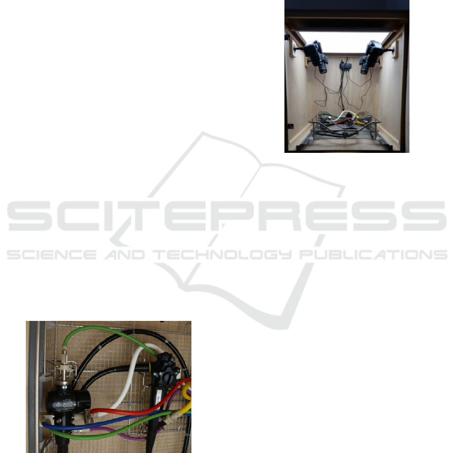
2.1 Hardware Setup
To accomplish the tasks of detecting errors in the
adaption, a complete prototype was built. The
system consists of a loading station wherein the
detection occurs and the integrated software which is
responsible for the processing pipeline of the
detection. As a basis for our image processing are
four images taken by four high-resolution cameras
from four different perspectives in order to capture
images without occlusions of relevant parts with a
high probability. Figure 1 shows an example of an
image which was taken by one of the cameras.
For optimal image processing it is important that
the scene is illuminated using controlled light
conditions (Bader, 2002). Because of that the
detection system is sealed in a cube to prevent
diffuse light entering the system. We enlighten the
detection system with a planar LED-Panel.
Camera sensors take 50% of the information
from the green interval of the spectrum. Green light
transfers approximately 72% of the luminance and is
there-fore most important for contrast and resolution
(Fukanaga, 1975) Because of that we chose an LED-
Panel with a color temperature of 6000 °K.
According to Wiens Law, the maximum radiation is
at 482.95 nm for 6000 °K which is within the green
part of the spectrum.
Figure 1: Example image of the scene, taken by one of the
four cameras.
The cameras are controlled using a serial interface
from the software to automate the system. With the
software we are also able to manipulate the settings
of the camera. So it is possible to adjust the aperture,
the ISO-value and the white balance. The white
balance is analogically set to 6000 °K. The other
values were set empirically , so that there is no over-
exposure and therefore no loss of information. We
use Canon EOS 750D cameras with a resolution of
24 Megapixel. A high resolution is essential for an
accurate detection.
Figure 2: Prototype.
We consider the task of detecting adaption errors
for a variety of different endoscopes and adapters. In
order to detect which endoscope is used, it is tagged
with an RFID chip. We use an RFID-reader, also
connected via a serial interface to differentiate
between them through their integrated RFID-tags.
On the basis of the detected endoscope the software
determines which and how many adapters should be
connected to the respective endoscope. The user gets
visual information on how to attach these adapters to
the detected endoscope. Figure 2 shows the general
setup of our prototype. At the front there is a door
which is not visible in the image.
2.2 Algorithmic Components
In order to classify whether an adapter is connected
correctly or not we use a pipeline of algorithms
which are explained in more detail in this chapter.
2.2.1 Image Registration
As explained in the introduction, we need to
measure the size of the gap between the two sides of
the adapter. We took several reference image pairs
of each adapter as shown in Figure
3.
HEALTHINF 2017 - 10th International Conference on Health Informatics
306
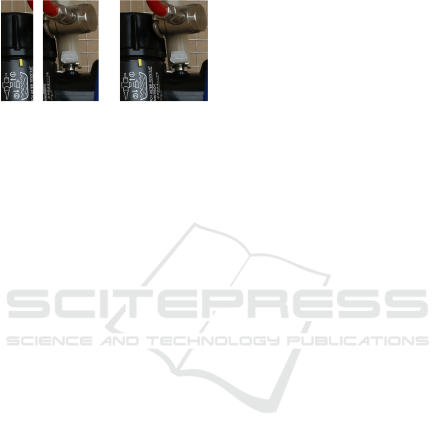
Figure 3: left: two parts of the same adapter, right: both
adapters matched together show a complete view of the
adapter.
If we combine those two parts of the image we get a
complete view of the adapter. Our goal is to map and
accordingly register these two-dimensional reference
images independently on a two dimensional
projection of the scene. For image registration, two
images are needed. The first is called reference
image denoted
, and the second is called template
image denoted
. This leads to a mathematical
optimization problem. We search for a linear
mapping :
→
that maps the object on
the
most exact to the object of
. Depending on the
class of transformations we can differentiate
between rigid, affine and perspective transformation.
The positions of the endoscope and thus the adapters
are completely unknown and only depend on the
employee of the hospital. Therefore, we are not able
to reach our goal with a simple rigid or affine
transformation. We have to describe a three-
dimensional transformation in space as a two-
dimensional projection in the image layer (Schreer,
2005). A projection like this is defined as an
endomorph description of a scene (Fischer, 2014).
A property of perspective projection is the loss of
proportions. Objects that are further away from the
center of projection appear smaller.
We can define this transformation as a 33
matrix
=
cos
sin
cos
1
(1)
which we apply to every position of the reference
image.
It is now known which form the transformation
matrix has to have to map a two-dimensional
reference image into the three-dimensional space
and map it again to a two-dimensional projection.
We have to determine the nine degrees of freedom
which uniquely define the matrix. To find the
required parameters, we need two sets of
corresponding points. is a set of points from the
reference image and ′ is a set of corresponding
points from the template image. Here
is the
transformation matrix of the perspective projection.
∙
=
⟺
=
′
(2)
To determine the transformation matrix we need
to have correspondences of points in the reference
and template image. In the following chapter we
show how these correspondences are detected.
2.2.2 Feature Detection
Feature detection algorithms are methods from the
field of computer vision. We use them to detect so
called interest points and correspondences between
points in two images. These images typically show
the same object, but at a different time or from a
different perspective. In the experiments we will
analyze two well established algorithms to examine
which one is more appropriate for this application
field. The two algorithms are the scale-invariant
feature transform (SIFT) (Lowe, 2004) and the
speeded up robust features (SURF) (Bay, 2008).
These two algorithms have the same general
process, which is divided into three steps: 1. feature
detection, 2. feature description and 3. feature
matching.
The first step, feature detection, deals with the
detection of so-called interest points. These are
distinctive points in an image. They always depend
on their neighborhood.
The feature description deals with the description of
the detected interest points, enabling a comparison
between the reference and the template images. The
most significant feature is the surrounding of one
point. Since the surroundings of the interest points
are never exactly the same on the reference and the
template image, a pixelwise comparison would not
work robustly. Furthermore, the descriptors have to
be invariant against geometric, perspective and
illumination transformations and image noise. Both
algorithms are based on computing one gradient of
the complete neighborhood of an interest point, as
well as in their sub regions.
The final step of the feature detection algorithms
matches interest points in the reference and template
image. The challenge is to find correct
correspondences of points, which in fact show the
same points of an object (Szeliski, 2011).
Every interest point is described through a
multidimensional description vector. A similarity
can be evaluated with the Euclidean distance
between the two descriptors. The most accurate but
slowest method is to compare every interest point of
Automatic Visual Detection of Incorrect Endoscope Adaptions in Chemical Disinfection Devices
307
the reference image with every interest point of the
template image. Since accuracy is one of our main
goals, we make use of this algorithm in the
experimental section. Other possibilities are the
randomized k-d tree (Silpa-Anan, 2008) and the
priority k-means tree algorithm (Fukanaga, 1975).
These algorithms are up to two times faster, approx-
imate to 95% of correctness (Muja, 2014).
Despite the high accuracy of SIFT and SURF,
there are always a few correspondence errors which
have to be filtered. We filter these errors with the
well-established random sample consensus
algorithm (RANSAC) (Strutz, 2016). If these errors
were not filtered they would have a bad influence on
the computation of the transformation matrix.
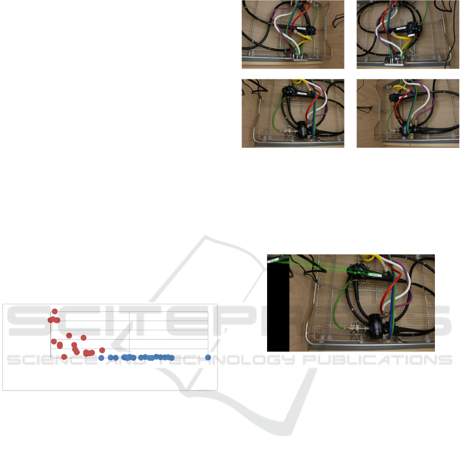
2.2.3 Machine Learning
To classify if an adapter is adapted correctly we use
a simple k-nearest neighbor approach. As features
we use the Euclidean distance between the two
projections and the number of detected corres-
pondences. Figure 4 shows an example of registered
features on one of the adapters. In this example the
classes are linear separable.
Figure 4: Normalized values of the Euclidean distances
and the number of correspondences, red: incorrect, blue:
correct.
2.2.4 Processing Pipeline
In this section we explain the complete processing
pipeline. Figure 5 shows four template images made
at runtime as explained previously.
We take five reference image pairs for every
adapter. One part of the pair shows the part of the
adapter at the endoscope, the other one the part of
the tube. The process is the same for every adapter.
Figure 5: Template images from four different
perspectives.
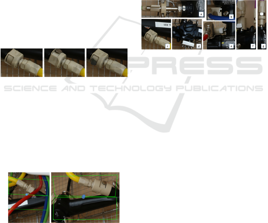
At first we intend to find the rough position of
the endoscope. For this purpose we use the feature
detection algorithm to find correspondences between
a reference image of the part of the adapter at the
endoscope.
Figure 6: Correspondence pairs between the reference
image and the template image to detect the rough position
of the adapter.
These interest points and correspondences are
easier to find because of the texts on the endoscope
which are very distinctive. We compute the mean of
all detected points in Figure 6 and crop that region
of the image depending on the size and geometry of
the adapter. This happens at a fourth of the
resolution to save time. The following computations
are made on the cropped images. This approach has
two advantages. First: The complex computations
are made on a much smaller image. Second: A
smaller image minimizes the probability of
correspondence errors.
When all subregions for all adapters were found,
the accurate registration of the reference image pairs
begins. For every adapter we have five reference
image pairs. As one can see in Figure 7 the adapters
not only have to be transformed in the space but may
have to be rotated longitudinally as well. For the
accurate registration we check all reference images
and choose the one with the most detected
0
0,2
0,4
0,6
0,8
1
00,51
Eucledean
Distance
Number of Correspondences
HEALTHINF 2017 - 10th International Conference on Health Informatics
308
correspondences.
Afterwards we detect and describe the interest
points of the chosen reference image of the adapter
on the side of the endoscope and the associated
reference image of the adapter on the side of the
tube. Then we identify correspondences between the
reference images and compute the transformation
matrices as shown in equations (1) and (2). With the
computed transformation matrices we map the
reference images into the template image we
identified previously. If the adaption is correct, the
projected reference images should intersect on the
inner edge as pictured in Figure 3. The same
matrices for mapping the reference images are used
to compute the center of the cutting edge. In Figure
8 one can see the two mapped reference images,
bounded in green rectangles. The midpoints of the
cutting edges are depicted by blue points. One can
recognize only one point at the left image because of
the optimal projections the two points overlap
completely. In the right image one can see an
incorrect adaption. The Euclidean distance between
the points is one feature for the classification of the
incorrect adaption.
Figure 7: A variety of reference images of the same
adapter because of the longitudinal rotations, which are
not detectable with the feature detection algorithms.
We use the two points to compute the Euclidean
distance between the two projections. An explorative
data analysis showed that the projection does not
work perfectly at all times. So it is not reliable as
single. Because of that we implemented a simple k-
nearest-neighbor Algorithm to classify the
adaptions. In addition to the Euclidean distance we
use the number of correspondences as a second
feature. This is depicted in Figure 4.
Figure 8: Mapped reference image pair on one template
image. The blue point marks the middle of their cutting
edges. Left: correct adaption, right: incorrect adaption.
3 EXPERIMENTAL RESULTS
As stated in the previous chapter, the detection of
interest points and correspondences is essential for a
correct projection of the reference images. The
quality of the transformation matrix is significantly
enhanced by detecting more correspondences. Vice
versa a faultless projection is impossible if there are
too many correspondence errors.. In this chapter we
describe the results of the detection processes and of
the classification.
We describe only the results of the reference
images on the side of the adapter. Because of the
high amount of letters on the endoscope itself, there
are a lot of interest points and the projection always
worked faultless.
Figure 9: Adapter set which we used for our experiments.
The quantitative results of the feature detection
algorithms are our first criteria for the quality of the
system. Figure
9
shows the adapter set we used for
our experiments. In the following tables we show the
statistic results of 40 processes for the first adapter
set. Table 1 shows the results for correct adaptions
generated with SURF.
The number of interest points and corres-
pondences - absolute and per pixel – is of special
importance here. In both categories one can see, that
the values are in the same order of magnitude for
most adapters. The adapters a, c, f and g have the
lowest values. This is because of the little body and
the few distinctive points on the adapters. So a
correct correspondence is more difficult to compute.
The adapters b, d and e have more distinctive points.
So the correspondences are easier to find. In Table 2
we see the statistical values for incorrect adaptions,
generated with SURF. The number of detected
interest points is similar. This makes sense, because
we use for both procedures images of the same size.
One can see the difference at the inspection of the
correspondences. For incorrectly adapted devices the
algorithm detects much less correspondences. This is
because the reference images were made with
correct adaptions.
Automatic Visual Detection of Incorrect Endoscope Adaptions in Chemical Disinfection Devices
309
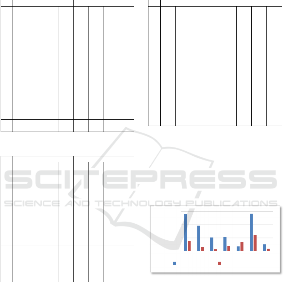
Table 1: Correct adaptions, generated with SURF as pre-
processor.
Interest Points Correspondences
Adapter
Mean #
Minimum #
Maximum #
Per Pixel
Mean #
Minimum #
Maximum #
Per Pixel
a
824
90
764 995
3.4
E-3
139
25
105 189
5.8
E-4
b
367
24
331 382
2.1
E-3
97
12
81 115
5.0
E-4
c
349
8
339 357
1.0
E-3
52
13
23 65
1.6
E-4
d
572
12
561 586
1.,9
E-3
53
6
45 63
1.7
E-4
e
107
3
106 117
1.9
E-3
17
10
9 43
3.0
E-5
f
111
6
82
883
114
2
3.4
E-3
142
21
114 114
4.0
E-4
g
441
33
371 465
2.0
E-3
26
6
18 35
1.1
E-4
Table 2: Incorrect adaptions, generated with SURF as pre-
processor.
Interest Points Correspondences
Adapter
Mean #
Minimum #
Maximum #
Per Pixel
Mean #
Minimum #
Maximum #
Per Pixel
a
794
33
780 888
3.3
E-3
38
16
24 73
1.6
E-4
b
356
26
323 382
2.0
E-3
15
5
10 25
8.0
E-5
c
342
6
339 354
1.0
E-3
7
2
5 10
2.0
E-5
d
566
29
540 602
1.8
E-3
19
9
12 40
6.0
E-5
e
159
58
106 227
2.8
E-3
35
38
4 86
6.0
E-5
f
873
31
0
142
114
2
3.0
E-3
60
27
27 91
1.8
E-4
g
424
49
324 465
1.9
E-3
9
4
7 19
4.0
E-5
If there is an incorrect adaption in the template
image it is possible, that there are large perspective
changes. If the perspective changes are too high, the
SURF algorithm cannot detect them, so fewer
correspondences are found as one can see in Figure
10. In six of the seven cases there are more than
twice as many detected correspondences. The only
exception here is adapter g because of its simple
structure and few interest points. These experimental
evaluations demonstrate that the number of
correspondences is a meaningful feature for the
machine learning algorithm.
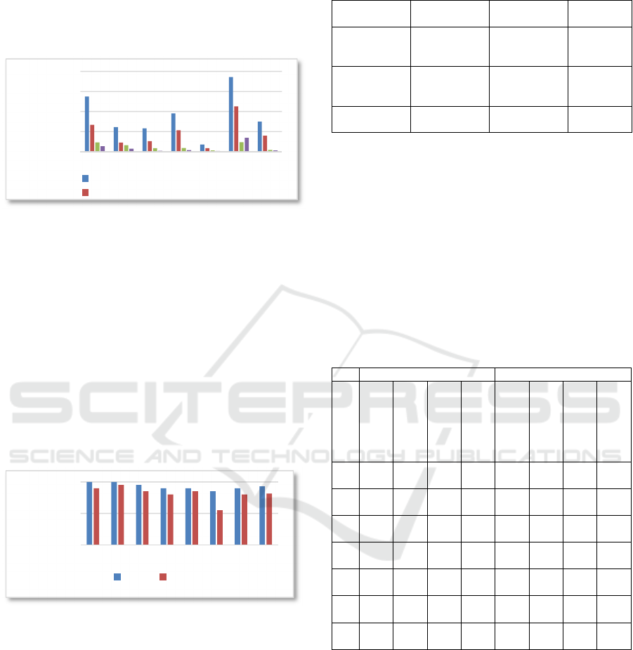
Table 3: Correct adaptions, generated with SIFT as pre-
processor.
Interest Points Correspondences
Adapter
Mean #
Minimum #
Maximum #
Per Pixel
Mean #
Minimum #
Maximum #
Per Pixel
a
402
5
391 407
1.7
E-3
80
13
54 91
3.3
E-4
b
135
8
121 140
8.0
E-4
46
5
38 51
2.6
E-4
c
157
13
140 170
5.0
E-4
14
5
7 26
1.0
E-5
d
321
20
278 336
1.0
E-3
23
7
15 33
7.0
E-5
e
52
8
41 58
9.0
E-4
9
3
5 13
1.5
E-4
f
697
18
5
206 776
2.0
E-3
208
10
191 220
6.3
E-4
g
238
40
199 339
1.0
E-3
17
5
10 28
7.0
E-5
In the following we outline the results of SIFT
for the same adapter set. The statistical values of
correct adaptions are shown in Table 3. Compared to
the SURF algorithm it attracts attention that SIFT
detects less interest points and correspondences than
SURF. The exact quotient is shown in Figure 11.
One can easily see that the SURF algorithm detects
more interest points and because of that more
Correspondences.
Figure 10: Comparison of the number of correspondences
between correct and incorrect adaptions.
In Table 5 one can see the statistical values for
incorrect adaptions, generated with SIFT. Analogue
to the SURF algorithm it is obvious that fewer
correspondences have been computed. This is
because of the similar procedure. Striking are the
detected minima of correspondences. If the
algorithm detects less than three correspondences, a
projection and following classification is impossible.
In summary we conclude, that the SURF algorithm
detects roughly twice as many correspondences than
0
50
100
150
abcdef g
Number of
Correspondeces
Correct - SURF Incorrect - SURF
HEALTHINF 2017 - 10th International Conference on Health Informatics
310
the SIFT algorithm. If we have too few corres-
pondences it is possible that the RANSAC algorithm
cannot filter the correspondence errors. The result is
an incorrect transformation matrix. Quantitatively
the SURF algorithm has to be preferred.
Figure 11: Comparison of the detected interest points and
correspondences.
Now we will focus on the quality and precision
of the classification. As outlined before we use a k-
nearest neighbor Algorithm for the binary
classification. The Euclidean distance of the
projection pairs and the number of correspondences
are the features of the algorithm. Experiments with
validation data gave us an optimal value for =5.
A first estimation of the quality of the processes
delivers the classification rate. In Figure 12 one can
see the classification rate per adapter for both
algorithms as pre-processing. All rates were
determined on test data experiments.
Figure 12: Comparison of the classification rates.
As predicted the process with SURF as pre-
processing has a significantly higher classification
rate of 92.86% compared to SIFT. The worst value
occurs at adapter e. This is because of the geometry
of the adapter. The Euclidean distance can be 0 for
this adapter although it is adapted incorrectly. This
adapter needs an additional physical rotation to be
correctly adapted. This can only be determined
through the number of detected correspondences.
Table 4: Confusion matrix of the classifications with
SURF as pre-processing.
SURF CORRECT
ADAPTIONS
INCORRECT
ADAPTIONS
PREDICTED
CORRECT
ADAPTIONS
TP = 64 FP = 4 P’ = 68
PREDICTED
INCORRECT
ADAPTIONS
FN = 6 TN = 66 N’ = 72
P = 70 N = 70
=140
Fawcett explains another possibility to evaluate
classifications (Fawcett, 2006). So called receiver
operating characteristics (ROC) graphs can be used
to evaluate and visualize the quality of a
classification. We divide the results of our experi-
ments in four groups: true-positive (TP), true-
negative (TN), false-positive (FP) and false-negative
(FN). These groups can be written in a so-called
confusion matrix (Fawcett, 2006), as one can see in
Table 4 and Table 6.
Table 5: Incorrect adaptions, generated with SIFT as pre-
processor.
Interest Points Correspondences
Adapter
Mean #
Minimum #
Maximum #
Per Pixel
Mean #
Minimum #
Maximum #
Per Pixel
a
339
5
397 409
1.7
E-3
40
9
24 51
1.6
E-4
b
136
7
121 140
8.0
E-4
10
6
3 19
5.0
E-5
c
160
35
140 256
5.0
E-4
5
2
3 8
1.0
E-5
d
317
21
278 336
1.0
E-3
18
6
9 30
5.0
E-5
e
131
99
41 246
2.3
E-3
26
25
3 76
4.6
E-4
f
711
10
5
557 776
2.2
E-3
142
53
44 209
4.3
E-4
g
203
14
190 239
9.0
E-4
8
3
4 13
3.0
E-5
The contents of the matrices were generated in 40
experiments and are a summary of all adapters. is
the number of correct, is the number of incorrect
adaptions. ′ is the number of positive, ′ is the
number of negative predictions. We can derive four
statistical values from these matrices: the true-
positive-rate (TPR), the false-positive-rate (FPR),
positive-predictive-value (PPV) and the accuracy
(ACC). We can now visualize the quality of the
classification with a ROC-Graph as shown in Figure
13.
0
300
600
900
1200
abcde fg
Count
Interest Points - SURF
Interest Points - SIFT
0%
50%
100%
abcdef gØ
classification
rate
SURF SIFT
Automatic Visual Detection of Incorrect Endoscope Adaptions in Chemical Disinfection Devices
311
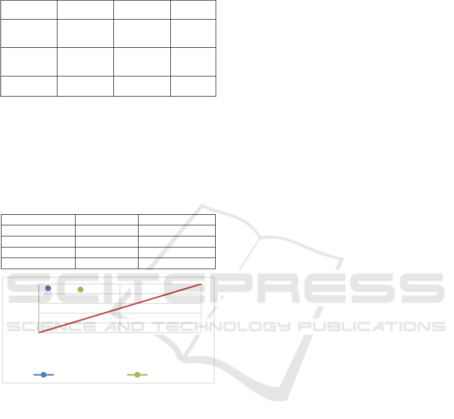
Table 6: Confusion matrix of the classifications with SIFT
as pre-processing.
SIFT CORRECT
ADAPTIONS
INCORRECT
ADAPTIONS
PREDICTED
CORRECT
ADAPTIONS
TP = 62 FP = 18 P’ = 80
PREDICTED
INCORRECT
ADAPTIONS
FN = 8 TN = 52 N’ = 60
P = 70 N = 70
=140
Ideally should the TPR be close to 1, the FPR close
to 0. The more the point is in the North-West, the
better is the classification. One can see in the
visualization that the processes with SURF as Pre-
Processing Algorithm is better than with SIFT. The
system needed in average 71/42 seconds for the
classification of the large/small adapter set.
Table 7: Statistical values from the confusion matrices.
SURF SIFT
TPR 0.914 0.886
FPR 0.057 0.257
PPV 0.941 0.775
ACC 0.928 0.814
Figure 13: ROC Graph.
4 CONCLUSION
This paper presents an automatic visual system for
detecting adaption errors in chemical disinfection
devices for endoscopes. Our experimental evaluation
shows promising results with respect to the
classification accuracy. With the SURF algorithm as
pre-processing tool, the prototype system yields a
classification accuracy of 92.86% for determining
the correctness of the adaptions in approximately
one minute of processing. Future work will aim in
enhancing the correctness of the prediction close to
100% and in installing the system directly into the
endoscope thermal disinfector to save even more
time and resources.
REFERENCES
Bader, L. et al, 2002 HYGEA (Hygiene in
Gastroenterology – Endoscope Reprocessing): Study
on Quality of Reprocessing Flexible Endoscopes in
Hospitals or Practice Setting. In Journal for
Gastroenterology 12 Pages 951-1000.
Muscarella, L., 2014 Risk of transmission of carbapanem-
resistant Enterobacteriaceae and related “superbugs”
during gastrointestinal endoscopy. In World Journal of
Gastrointestinal Endoscopy 6 Pages 951-1000.
Handels, H., 2009. Medizinische Bildverarbeitung,
Vieweg und Teubner. Wiesbaden, 2
nd
edition.
Zitova, B., Flusser, J., 2003. Image registration methods: a
survey. In Image and Vision Computing Volume 21
Pages 977-1000.
Lowe, D, 2004, Distinctive Image features from Scale-
Invariant Keypoints. In International Journal of
Computer Vision 60 Pages 91-110.
Bay, H. et al, 2008, Speeded-Up Robust Features (SURF).
In Computer Vision and Image Understanding Pages
346-359.
Schreer, O., 2005. Stereoanalyse und Bildsynthese,
Springer Verlag. Berlin Heidelberg, 1
st
edition.
Fischer, G., 2014. Lineare Algebra, Springer Verlag.
Berlin Heidelberg, 18
th
edition.
Szeliski, R., 2011. Computer Vision, Springer Verlag.
Berlin Heidelberg, 1
st
edition.
Silpa-Anan, C., Hartley, 2008, R., Optimised KD-Tree for
fast image descriptor matching. In Computer Vision
and Pattern Recognition
Fukanaga, K., Narendra, P., 1975, A branch and bound
Algorithm for Computing k-Nearest Neighbors. In
IEEE Transactions on Computers C-24 Pages 750-
753.
Muja, M., Lowe, D., 2014, Scalable Nearest Neighbor
Algorithms for High Dimensional Data. In IEEE
Transactions on Pattern Analysis and Machine
Intelligence 36 Pages 2227-2240.
Strutz, T., 2016. Data Fitting and Uncertainty, Springer
Verlag. Berlin Heidelberg, 2
nd
edition.
Fawcett, T., 2006, An introduction to ROC Analysis. In
Pattern Recognition Letters 27 Pages 861-874.
0
0,2
0,4
0,6
0,8
1
00,51
true positive rate
false positive rate
ROC - SURF ROC - SIFT
HEALTHINF 2017 - 10th International Conference on Health Informatics
312
