
Line-based SLAM Considering Directional Distribution of Line Features
in an Urban Environment
Kei Uehara
1
, Hideo Saito
1
and Kosuke Hara
2
1
Graduate School of Science and Technology, Keio University,
3-14-1 Hiyoshi Kohoku-ku, Yokohama, Kanagawa, 223-0061, Japan
2
Denso IT Laboratory, Cross Tower 28F, 2-15-1 Shibuya Shibuya-ku, Tokyo, 150-0002, Japan
{kei-uehara, saito}@hvrl.ics.keio.ac.jp, khara@d-itlab.co.jp
Keywords:
Line-based SLAM, Manhattan World Assumption, Road Markings, Gaussian Distribution.
Abstract:
In this paper, we propose a line-based SLAM from an image sequence captured by a vehicle in consideration
with the directional distribution of line features that detected in an urban environments. The proposed SLAM
is based on line segments detected from objects in an urban environment, for example, road markings and
buildings, that are too conspicuous to be detected. We use additional constraints regarding the line segments
so that we can improve the accuracy of the SLAM. We assume that the angle of the vector of the line segments
to the vehicle’s direction of travel conform to four-component Gaussian mixture distribution. We define a
new cost function considering the distribution and optimize the relative camera pose, position, and the 3D
line segments by bundle adjustment. In addition, we make digital maps from the detected line segments. Our
method increases the accuracy of localization and revises tilted lines in the digital maps. We implement our
method to both the single-camera system and the multi-camera system. The accuracy of SLAM, which uses
a single-camera system with our constraint, works just as well as a method that uses a multi-camera system
without our constraint.
1 INTRODUCTION
Currently, advanced driver assistance sys-
tems(ADAS) has been actively researched. An
autonomous car is an example of an ADAS that will
enable people to go anyplace without your driving
operation.To achieve that, it requires localization to
calculate its’ trajectory. (Teramoto et al., 2012) indi-
cated that the accuracy of the localization required
for practical use is from several dozen centimeters
to several meters. For localization, one of the main
methods is to use GPS. Although POSLV, one of
the high-end integrated accurate positioning system,
achieves accuracy within several dozen centimeters
using a RTK-GPS receiver, it is not appropriate for
use in the autonomous car. One reason is that the cost
of RTK-GPS is very high. Another reason is that the
GPS system depends on the strength of microwaves
from the satellite. Thus, if the vehicle is in the tunnel,
it cannot work.
Meanwhile, the visual simultaneous localization
and mapping system (SLAM) has been attracting at-
tention of researchers because it does not have these
problems. To determine its position, detects feature
points from the environment around the vehicle us-
ing a camera as an input. In the case that feature
points can be detected fully, the accuracy of SLAM
is as well as a method with laser range scanner. Since
the accuracy of SLAM decreases without enough fea-
ture points, there are many studies trying to solve that
problem; for example, studies that uses multi-cameras
or researches detect not only points, but also lines.
However, using many feature points or lines means an
increasing of calculation cost, and it is fatal because
the system of the autonomous car requires a real-time
calculation. Increasing equipment means increasing
of production costs. The less equipment attached to
the vehicle, the better it is as long as the accuracy is
maintained in the autonomous car.
In this paper, we propose a line-based SLAM con-
sidering a directional distribution of line features in
an urban environment, which is based on the Manhat-
tan world assumption. Based on the fact that many
line segments in road markings are parallel or vertical
to a vehicle’s direction of travel, we define the distri-
bution as four-component Gaussian mixture distribu-
tion. To prove our method’s effectiveness, we con-
duct four experiments: 1) single-camera system with
line-based SLAM, 2) multi-camera system with line-
Uehara K., Saito H. and Hara K.
Line-based SLAM Considering Directional Distribution of Line Features in an Urban Environment.
DOI: 10.5220/0006149302550264
In Proceedings of the 12th International Joint Conference on Computer Vision, Imaging and Computer Graphics Theory and Applications (VISIGRAPP 2017), pages 255-264
ISBN: 978-989-758-227-1
Copyright
c
2017 by SCITEPRESS – Science and Technology Publications, Lda. All rights reserved
255
based SLAM, 3) single-camera system with line-and-
point-based SLAM, and 4) multi-camera system with
line-and-point-based SLAM. We can achieve a high
accuracy of SLAM in all experiments by our method.
In addition, we simultaneously make a digital
map. Although, the digital map has been used in
ADAS, it must be accurate and up-to-date. Roads and
road markings are destroyed frequently, so they must
be updated. Our digital map can be generated while
driving on streets, and it requires cameras. No other
equipments are needed. SLAM often has some intrin-
sic or extrinsic errors, so the line segments in the map
often tilt. However, it is not a problem in our method
because the directional distribution is considered.
2 PREVIOUS WORKS
Our goal is to realize SLAM using the distribution of
line segments. There are some SLAM works that use
line and road markings. Therefore, we discuss line-
based SLAM and SLAM using road markings sepa-
rately in this section.
2.1 Line-based SLAM
There are previous works on line-based SLAM that
have taken different approaches. (Smith et al., 2006)
proposed a real-time line-based SLAM. They added
straight lines to a monocular extended Kalman filter
(EKF) SLAM, and realized the real-time system using
a new algorithm and a fast straight-lines detector that
did not insist on detecting every straight line in the
frame.
Another approach for the line-based SLAM is us-
ing lines and other features. (Koletschka et al., 2014)
proposed a method of motion estimation using points
and lines by stereo line matching. They developed a
new stereo matching algorithm for lines that was able
to deal with textured and textureless environments.
In addition, (Zhou et al., 2015) proposed a vi-
sual 6-DOF SLAM (using EKF) based on the struc-
tural regularity of building environments, which is
called the Manhattan world assumption (Coughlan
and Yuille, 1999). By introducing a constraint about
buildings, the system achieved decreasing position
and orientation errors.
2.2 SLAM using Road Markings
There are also previous works using road markings
for SLAM for a vehicle. (Wu and Ranganathan, 2013)
proposed a method for SLAM using road markings
that they previously learned. They detected feature
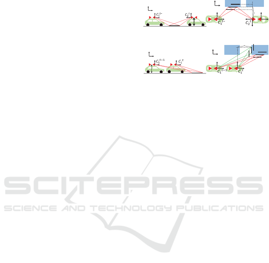
Yw
Zw
h
s
(a) On roads (inter)
Xw
Zw
dx
s
(b) On buildings (inter)
Yw
Zw
h
(c) On roads (intra)
Xw
Zw
dz
(d) On buildings (intra)
Figure 1: Examples of intra- and inter-camera correspon-
dences.
points from learned road markings and achieved a
high accuracy in estimation of a camera pose.
(Hata and Wolf, 2014) proposed a method which
detects road markings robustly for SLAM. They de-
veloped a line detector which did not affected by il-
lumination condition by adapting Otsu thresholding
method.
In addition, (Z.Tao et al., 2013) combined GPS,
proprioceptivesensors, and road markings for SLAM.
3 SYSTEM OVERVIEW
We provide an overview of a line-based SLAM con-
sidering the distribution of road markings. We im-
plement our method into both a single-camera system
and a multi-camera system. We explain the method of
the multi-camera system because the radical method
for both the single-camera and the multi-camera sys-
tems is the almost same .
As a premise, our SLAM method requires wheel
odometry. A relativecamera pose and position in each
frame are estimated from the data from the wheel sen-
sors. Then, we obtain line segments from input im-
ages for each frame t by the line segment detector
(LSD) algorithm. To correspond detected line seg-
ments, we consider the following three cases: match-
ing between the front images features at frame t and
t − 1, matching between the rear image at frame t
and t − 1, and matching between the rear image at
frame t and the front image at frame t − s. However,
the viewing directions are very different, so it is hard
to find matching segments, especially in the case of
the third case. For a robust match, we make the fea-
ture patches around the line segments warp into other
frames. Due to this warping processing, the perspec-
tive appearance of the patch resembles a target image.
In addition, searching for the appropriate s value for
the best match enables us to find the correspondences
VISAPP 2017 - International Conference on Computer Vision Theory and Applications
256

between a rear image and multiple front images more
robustly. As long as corresponding line segments are
detected, each line segment can be tracked over. Fig-
ure 1 indicates examples of matching.
Using these corresponding line segments, 3D line
segments can be initially estimated using a method
based on the Manhattan world assumption. After
that, bundle adjustment is applied to the relative cam-
era pose, positions and 3D line segments to optimize
them. In a cost function of bundle adjustment, which
is used for the optimization, we implement a new el-
ement considering the distribution of road markings,
which is defined by 4-component Gaussian mixture
distribution. Due to this element, the accuracy of lo-
calization improves and tilted line segments, which
include some errors, in the generated map are revised.
The difference between a single-camera system
and a multi-camera system is that the former does not
consider the third matching case: matching between
the rear image at frame t and the front image at frame
t − s.
4 NOTATION
We explain the notations briefly before discussing our
method in detail. First, we define the four coordi-
nates W, C
1
t
, C
2
t
and V
t
, which indicate the world,
front camera, rear camera, and vehicle coordinate sys-
tems, respectively. The relative transformations from
the world coordinate system to the vehicle coordi-
nates system at frame t are expressed as R
vw
t
, T
vw
t
,
and these from the vehicle coordinates system to the
front or the rear camera coordinate system are ex-
pressed as R
c
1
v
, T
c
1
v
, R
c
2
v
, T
c
1
v
. The relative pose
and position of the front and rear cameras are cali-
brated beforehand. Using these notations, the projec-
tions from a world point p = (x,y,z)
T
to camera point
q = (q
x
,q
y
,q
z
)
T
are calculated as follows:
q
k
=
q
x
q
y
q
z
= R
c
k
v
(R
vw
t
p+ T
vw
t
) + T
c
k
v
(1)
where k denotes camera 1 or camera 2. For this case,
k = 1 indicates the front camera. Then, projection
from a camera point q to a image point u = (u,v)
T
is
calculated as follows:
u
k
=
u
v
= π
q
x
q
y
q
z
=
q
x
/q
z
q
y
/q
z
(2)
Secondly, the 3D line L
k
is expressed as six-vector
(p
k
T
,r
k
T
)
T
. The three-vectors p
k
is a center point of
the 3D line and r
k
is the direction of the 3D line. The
2D line l
k
, which is a projection line of L
k
in the im-
age plane, is given as four-vector (u
k
T
,d
k
T
)
T
. Point
u is calculated in the same way as the world point p
and the vector d in the image plane is calculated as
follows:
D
k
=
D
x
D
y
D
z
= R
c
k
v
R
vw
t
r
k
(3)
d
k
=
d
x
d
y
=
q
z
D
x
− q
x
D
z
q
z
D
y
− q
y
D
z
(4)
where D
k
is a point of the camera coordinate system.
Finally, the wheel odometry x is expressed as follows:
x
t+1
=
x
t+1
z
t+1
θ
t+1
= x
t
+ ∆x
t
+ ε
x
t
(5)
where ∆x
t
denotes its relative movement from a pre-
vious time and ε
x
t
denotes the noise of ∆x
t
. In the
proposed method, we estimate the 3-DOF motion of
the vehicle coordinates (x, z, θ) in a 2D-environment.
When x
0
, which is the initial position of the vehicle,
is in the same position as the origin of the world coor-
dinate system, x
t
equals R
vw
t
and T
vw
t
. We suppose
that ε
x
t
is zero-mean Gaussian white noise with co-
variance Σ
x
.
ε
x
t
∼ N (0,Σ
x
) (6)
Σ
x
=
σ
x
2
0 0
0 σ
z
2
0
0 0 σ
θ
2
∆t (7)
where σ
x
, σ
z
, and σ
θ
denote error variances. The con-
variance increases in proportion to time, supposing
that ε
x
t
simply increases.
5 PROPOSED METHOD
The purpose of our method is to enhance the accuracy
of line-based SLAM by bundle adjustment, which
considers the distribution of the line segments. Our
system consists of two parts: line matching and bun-
dle adjustment. In this section, we explain how to
realize them individually.
5.1 Line Matching
Our method has two matching algorithms: match-
ing inter-camera correspondences and matching intra-
camera correspondences, the basis of which is warp-
ing patches based on the Manhattan world assump-
tion. We explain them individually.
Line-based SLAM Considering Directional Distribution of Line Features in an Urban Environment
257
5.1.1 Inter-Camera Correspondences
This method of matching is used between the front
and the rear images, and is not featured with a single-
camera system. The blue-colored rectangle shown in
Figure 2(a) is a patch, which is 20 pixels wide and
has a detected red-colored line segment in the center.
The patch is transformed into a target image plane by
a warp function, which considers the place where the
line segments are detected. Conceivable places where
they can be detected include front walls of buildings
or road surfaces, as shown in Figure 1(a) and (b).
Therefore, two types of warping processing are per-
formed on all line segments in this matching algo-
rithm.
To explain the case of the front walls of building,
according to the Manhattan world assumption, a y-
coordinate value of all the points in the patch in C
2
t
is
h, which indicates the height of the attached camera.
Therefore, the 3D point in the patch is calculated as
follows:
p
r
=
h(u
m,2
+ α)/(v
m,2
+ β)
h
h/(v
m,2
+ β)
(8)
We define the coordinate of the patch as u
m,2
=
(u
m,2
+ α,v
m,2
+ β)
T
, where u
m,2
denotes the center
point of the line segment and α and β are the Eu-
clidean distances from the center point.
In the case of the line segments detected on the
road surface, the 3D point in the patch is calculated as
follows:
p
bf
=
d
x
d
x
(v
m,2
+ β)/(u
m,2
+ α)
d
x
/(u
m,2
+ α)
(9)
The x-coordinate value of all the points in the patch
in C
2
t
is d
x
, which is shown in Figure 1(b), under the
assumption.
The result of the warping is shown in Figure
2(b). It shows that the perspective appearance be-
comes similar to the target image (Figure 2(c)). Sub-
sequently, we judge whether the warped patch and the
line segments in the target image correspond or not
with using an error ellipse based on the EKF proposed
by (Davison et al., 2007). We use a raster scan of the
error ellipse of the warped patch and calculate a zero-
mean normalized cross-correlation (ZNCC) score. At
the position where the ZNCC is the highest, we calcu-
late two more values: the angle between the warped
line segment and the line segments in the target im-
age, and the distances from the endpoints of warped
line segments to the line segment in the target image.
If these two values are lower than the threshold, they
are regarded as the correspondence.
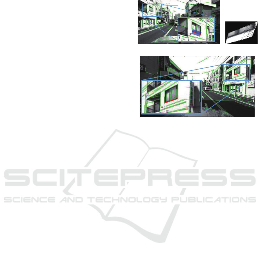
(a) Rear image and patch (b)Warped patch
(c) Front image and a detected line segments
Figure 2: (a)A rear image with a patch of the red detected
line. (b) The warped patch converted from (a). (c) The front
image.
Although we propose this matching method, it has
two ambiguous points: one is that we cannot precisely
distinguish whether the line segments exist on build-
ings or the road surface, and the precise value of d
x
cannot be calculated. To exclude these ambiguous
elements, we test two calculations, for the building
and road surface, and change d
x
at regular intervals in
each experiment. Then we decide the correspondence
based on the highest ZNCC score.
5.1.2 Intra-Camera Correspondences
This method of matching is used between pairs of
front images or pairs of rear images. There are three
conceivable places where the line segments can be de-
tected in this method: two of three are the same as the
inter-camera correspondences and the last one is the
side wall of buildings, as shown inFigure 1(c) and (d).
The 3D point in the patch is calculated as follows:
p
bs
=
d
z
(u
m,1
+ α)
d
z
(v
m,1
+ β)
d
z
(10)
Under the Manhattan world assumption, z-coordinate
of all the 3D points in the patch is d
z
, which is shown
in Figure 1(b), so Equation 10 can be defined. As well
as the inter-camera correspondences, we change d
z
at
regular intervals and find the best one for matching.
5.1.3 The Matching Result
The results of matching are shown in Figures 3.
VISAPP 2017 - International Conference on Computer Vision Theory and Applications
258
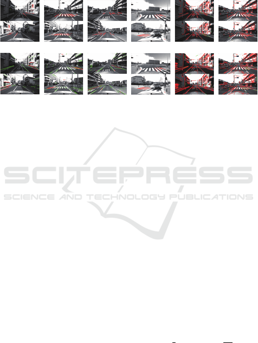
(a) (b) (c) (d) (e) (f)
(g)
(h) (i)
(j)
(k) (l)
Figure 3: Examples of matching using our method (a)-(f) and LEHF (Hirose and Saito, 2012) (g)-(l). (a)-(d) and (g)-(j) are
matched pairs of front and rear images. (e) (f), (k), and (l) are matched pairs of front images. The red lines and green lines
show correct and incorrect matching, respectively.
Figures 3(a) to (d) indicate intra-matching corre-
spondences with using our method, and Figure 3(g)
to (j) indicate correspondences using LEHF (Hirose
and Saito, 2012). Although, the enough number of
the line segments cannot detected, the accuracy of the
matching obviously increases.
Figures 3(e) and (f) indicate inter-matching corre-
spondences with using our method, and Figures 3(k)
and (l) indicate correspondences using LEHF (Hirose
and Saito, 2012). The accuracy of them is the almost
same.
Using our method, we can classify all matched
line segments into on the building walls or
on the road, which LEHF cannot do. This detected
place data are important for the next step.
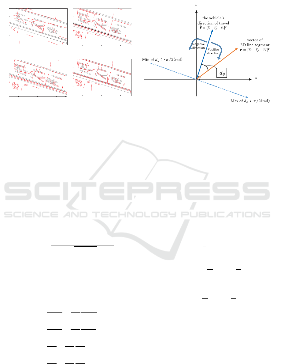
5.2 Initial Estimation of 3D Line
We use two methods to estimate the 3D line segments,
which will be explained individually in this section.
First, we estimate line segments using a method
based on the line of intersection of planes that passes
the camera center and the line segment. Figure 4(a)
shows examples of road maps generated by the 3D in-
formation calculated by this method, although most of
them lie wrong place. The reason for this is because
when the line segments run parallel to the travel di-
rection, the angle between the plane passing the seg-
ments becomes too low. The 3D information create
error because of that.
Secondly, we estimate the line segments using
Equations (8)(9),(10) as explained in Section 5.1. In
this method, we can obtain some 3D information per
one line segment, because it requires only one line
segment to calculate the 3D information and each
line segment has some corresponded line segments.
Therefore, we choose one line segment by minimum
median method. An element used in the minimum
median method is the re-projection error,which is cal-
culated from the perpendicular distance from a repro-
jected 3D line to the endpoints of a detected line in the
image plane. This method is widely used and is de-
fined in a paper written by (Bartoli and Sturm, 2005).
Figure 4(b) shows a result of this method, which is
obviously better than first method.
5.3 Optimization by Bundle Adjustment
We optimize the relative camera pose, position (R
vw
t
,
T
vw
t
) and the 3D line segments L
j
by bundle adjust-
ment. We define the set of corresponding line seg-
ments Ω as :
Ω ={ω
i
= (t,k, j, p)|
t ∈ {1,...,T},k ∈ {1,2}, j ∈ {1,...,J} p ∈ {1,2,3}}
(11)
where the ith line segment indicates that a 3D line
is observed in a place p by camera k at frame t. In
our method, the objectives are to minimize the re-
projection errors of all the line segments and to mini-
mize the angle errors of the line segments observed in
the road surface. Then, the cost function is defined as
following.
E = e
2
l
+ e
2
θ
=
1
2
∑
i
2
∑
n=1
d
2
⊥
(g
n
i
,l
i
) +
1
2σ
2
∑
m
(e
θ
m
)
2
(12)
Line-based SLAM Considering Directional Distribution of Line Features in an Urban Environment
259
]>P@
[>P@
(a) Standard initial estimation
]>P@
[>P@
(b) Our initial estimation
]>P@
[>P@
(c) Without the constraint
]>P@
[>P@
(d) With the constraint
Figure 4: Examples of road maps.
where d
⊥
(a,b) denotes the perpendicular distance
from a point a to a line b in images, g
1
i
and g
2
i
de-
note the endpoints of observed line segments, and e
θ
denotes an angle error, which can be calculated using
the difference between the travel direction of the vehi-
cle and the vector of the line segments. An objective
is to find the best values of R
vw
t
, T
vw
t
, and L
j
to min-
imize E. We use the iterative non-linear Levenberg-
Marquardtoptimization algorithm with numerical dif-
ferentiation based on a method proposed by (Madsen
et al., 1999). We explain the calculation method for
the reprojection error and angle error individually.
5.3.1 Reprojection Error
We use the following equation to calculate d
⊥
(g
n
i
,l
i
):
e
i
l
= d
⊥
(g
n
i
,l
i
) =
d
y
(g
x
i
− u
i
) − d
x
(g
y
i
− v
i
)
q
d
x
2
+ d
y
2
(13)
To solve the bundle adjustment, we make Jacobian
matrices made from the result of differentiated Equa-
tion (13) in the relative camera pose, position(R
vw
t
,
T
vw
t
) and the 3D line segments L
j
. The differentia-
tion equations are expressed as follows by conform-
ing to the chain rule:
∂e
l
i
∂R
vw
t
=
∂e
l
i
∂q
i
∂q
i
∂R
vw
t
(14)
∂e
l
i
∂T
vw
t
=
∂e
l
i
∂q
i
∂q
i
∂T
vw
t
(15)
∂e
l
i
∂p
j
=
∂e
l
i
∂q
i
∂q
i
∂p
j
(16)
∂e
l
i
∂r
j
=
∂e
l
i
∂D
i
∂D
i
∂r
j
(17)
where q and D are defined as Equations (1) and (4),
respectively.
.
Figure 5: A schematic diagram of d
θ
.
In addition, we include a geometric constraint into
the cost function to enhance the accuracy of the opti-
mization. Under the Manhattan world assumption, y-
coordinate of the line segments detected on the road
surface is absolutely h, so we keep it constant dur-
ing the process of bundle adjustment. Since d
x
and
d
z
have ambiguousness, we do not incorporate that
constraint. Figure 4(c) and (d) are the result of map-
ping after bundle adjustment without or with the con-
straint, respectively. The figures show that the con-
straint works well.
5.3.2 Angle Error
First, we show that d
θ
in Figure 5 is an angle between
the travel direction and the vector of the 3D line seg-
ments, and it has either a positive or a negative value;
the maximum value is
π
2
and the minimum value is
−
π
2
. It is calculated as follows:
d
θ
= arctan
F
z
F
x
− arctan
r
z
r
x
(18)
((F
x
≧ 0 and F
z
≧ 0) or (F
x
≦ 0 and F
z
≦ 0))
d
θ
= arctan
F
z
F
x
− arctan
r
z
r
x
− π (19)
((F
x
≧ 0 and F
z
≦ 0) or (F
x
≦ 0 and F
z
≧ 0))
where F = (F
x
,F
y
,F
z
) denotes the vehicle’s direction
of travel. To establish the consistency of the sign
of d
θ
, we take π from d
θ
in Equation (19). In our
method, we add a new constraint about d
θ
. As I dis-
cussed in section 1, we suppose that most of the road
markings are parallel or vertical to the vehicle’s direc-
tion of travel. Although some markings include diag-
onal lines, there are many markings that include paral-
lel or vertical lines; for examples, car lanes, and mark-
ings at crosswalks. In the case of the parallel line, we
VISAPP 2017 - International Conference on Computer Vision Theory and Applications
260
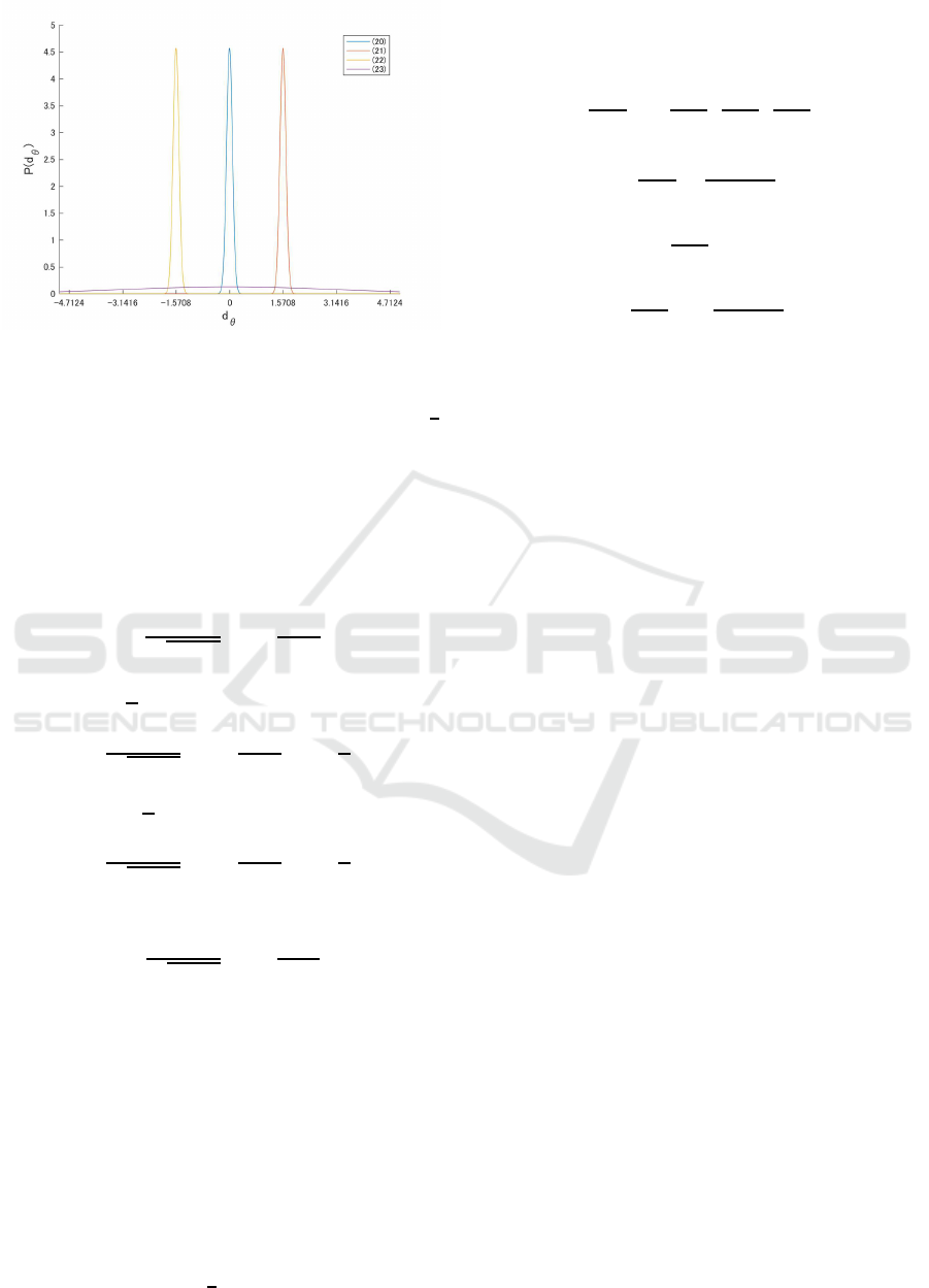
Figure 6: A four-component Gaussian mixture distribution.
assume that d
θ
conforms to the Gaussian distribution.
In the case of the vertical line, we assume that d
θ
±
π
2
conforms to the Gaussian distribution. Figure 6 shows
their distribution. Considering the diagonal lines, we
define one more Gaussian distribution. It prevents the
diagonal lines from being corrected to the parallel or
vertical lines. The equations can be expressed as fol-
lows:
P
1
(d
m
θ
|µ = 0,σ = σ
α
) =
1
p
2πσ
α
2
exp(−
1
2σ
α
2
(d
m
θ
)
2
)
(20)
P
2
(d
m
θ
|µ =
π
2
,σ = σ
α
) =
1
p
2πσ
α
2
exp(−
1
2σ
α
2
(d
m
θ
−
π
2
)
2
)
(21)
P
3
(d
m
θ
|µ = −
π
2
,σ = σ
α
) =
1
p
2πσ
α
2
exp(−
1
2σ
α
2
(d
m
θ
+
π
2
)
2
)
(22)
P
4
(d
m
θ
|µ = 0,σ = σ
β
) =
1
q
2πσ
β
2
exp(−
1
2σ
β
2
(d
m
θ
)
2
)
(23)
The numbers in the Legend of Figure 6 correspond to
these equations.
Based on these equations, the cost function is cal-
culated as follows:
e
m
θ
= d
θ
− µ (24)
This equation indicates that if the line segment is ver-
tical, but is a little tilted, it is corrected to the accurate
vertical line; and if it is parallel, but is a little tilted, it
is corrected to the accurate parallel line. The value of
µ is decided by the value of P(d
θ
); if P
2
(d
θ
) is greater
than other P values, µ is
π
2
.
As well as reprojection error, we make a Jacobian
matrix. The differentiated equations are expressed as
follows:
∂e
θ
j
∂r
=
∂e
θ
j
∂r
x
∂e
θ
j
∂r
y
∂e
θ
j
∂r
z
(25)
∂e
θ
j
∂r
x
=
r
z
r
x
2
+ r
z
2
(26)
∂e
θ
j
∂r
y
= 0 (27)
∂e
θ
j
∂r
z
= −
r
x
r
x
2
+ r
z
2
(28)
In addition, we obtain the best value of σ
α
and
σ
β
by changing them at regular intervals for the best
optimization in each experiment.
6 EXPERIMENT
In this section, we introduce a practical experiment
that uses a real vehicle driving in an urban environ-
ment. Two cameras and a RTK-GPS, which can get
high accuracy of self-position, are attached to the ve-
hicle. The frame rate of the camera is 10 fps and
we prepare two datasets: one is a straight scene that
has 72 frames and another is curve scene that has 200
frames. We use the GPS as a ground truth. We evalu-
ate the accuracy of localization and mapping individ-
ually.
6.1 Evaluation of Localization
In our experiment, we apply our method to four cases;
1) single-camera system with line-based SLAM
(called line (S)), 2) single-camera system with point-
and-line based SLAM (point-line (S)), 3) multi-
camera system with line-based SLAM (line (M)),
and 4) multi-camera system with point-and-line based
SLAM (point-line (M)). We check how much the ac-
curacy of localization improves when the directional
distribution of road markings is considered in each
cases.
Figure 7 shows trajectories of the vehicles in the
case of line (S) in two datasets. We compare four
types of data in each case; ground truth, odome-
try, optimized data without the directional constraint,
and optimized data with the directional constraint. A
closeup area (1) of Figure 7(a) and (b) indicates that
the optimized data with the constraint is the closest
to the ground truth and it has higher accuracy than
that without the constraint. However, (2) of Figure
7(a) indicates the accuracy decreases by adding the
Line-based SLAM Considering Directional Distribution of Line Features in an Urban Environment
261
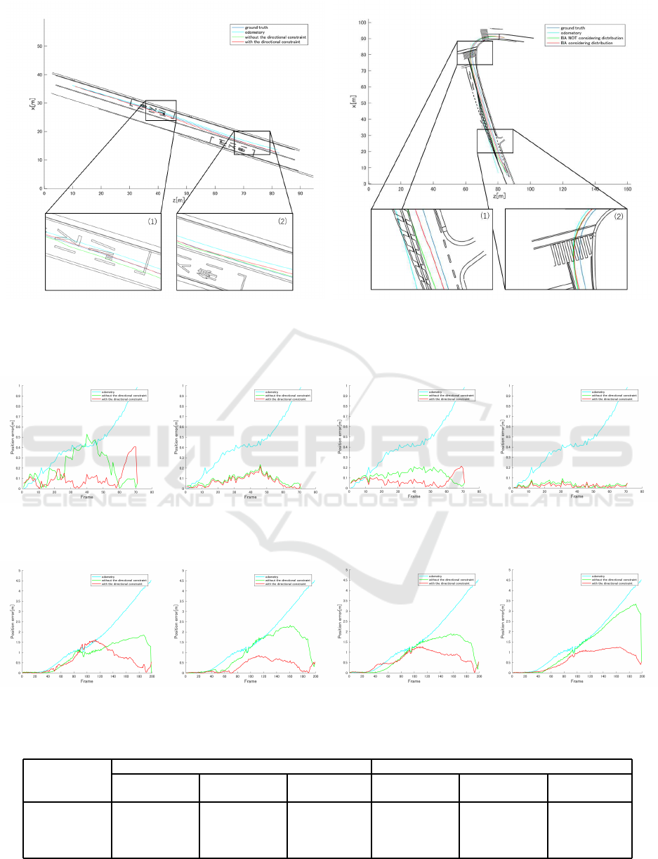
(a) Dataset 1
(b) Dataset 2
Figure 7: The trajectory results obtained from datasets 1 and 2 in the experiment of line (S). Comparison of the results
estimated by ground truth, odometry, optimized data without the constraint, and optimized data with the constraint
(a) line (S) (b) line (M)
(c) line-point (S) (d) line-point (M)
Figure 8: Comparison of position error in each frame (dataset 1).
(a) line (S) (b) line (M)
(c) line-point (S) (d) line-point (M)
Figure 9: Comparison of position error in each frame (dataset 2).
Table 1: The sum of the position error and the improvement rate.
Dataset 1 Dataset 2
Without the
constraint [m]
With the
constraint [m]
Improvement
rate [%]
Without the
constraint [m]
With the
constraint [m]
Improvement
rate [%]
line (S) 13.57 6.52 52.0 176.11 107.32 39.1
line (M) 6.22 5.54 10.9 205.56 65.16 68.3
line-point (S) 8.45 4.32 48.9 186.18 125.96 32.3
line-point (M) 2.62 1.58 39.7 267.90 129.20 51.8
VISAPP 2017 - International Conference on Computer Vision Theory and Applications
262
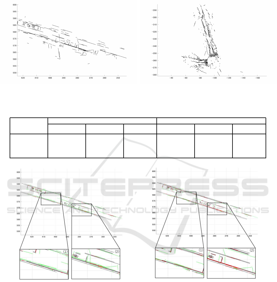
(a) Dataset 1 (b) Dataset 2
Figure 10: Digital maps made from detected line segments.
Table 2: The rate of inlier lines
Dataset 1 Dataset 2
Without the
constraint [%]
With the
constraint [%]
Change [%]
Without the
constraint [%]
With the
constraint [%]
Change [%]
line (S) 28.5 47.5 +19 40.1 35.9 -4.2
line (M) 35.1 41.6 +6.5 39.6 36.9 -2.7
line-point (S) 39.1 49.7 +10.6 41.5 33.4 -8.1
line-point (M) 49.6 52.8 +3.2 42.2 39.1 -3.1
(a) Without the constraint (b) With the constraint
Figure 11: Mapping results in line (S) Red lines indicate inliar lines and green lines indicate outlier lines.
constraint. The reason for that is because the vehicle
cannot detect enough line segments. Actually, there
are few line segments in the area.
Figure 8 and Figure 9 provide a quantitative anal-
ysis of the accuracy of localization. They are posi-
tion errors, which indicate a perpendicular distance
to the ground truth. In addition, Table 1 shows the
sum of the position errors in each case and the rate of
improvement in percentage. The accuracy improves
in all experiments by considering the constraint. For
dataset 1, the accuracy improves about 50% in the
single-camera experiment. The accuracy of line (S)
with the constraint is as well as line (M) without it.
For dataset 2, the accuracy improves, especially in the
multi-camera experiments. Since our SLAM method
is based on the Manhattan world assumption, it is not
appropriate for the curving scene because the assump-
tion does not stand up well . However, by using the
Line-based SLAM Considering Directional Distribution of Line Features in an Urban Environment
263

directional constraint, the error generated in the curv-
ing scene is revised. It may be a reason for the high
improvement rate seen in dataset2.
6.2 Evaluation of Mapping
The detected line segments can be used to make dig-
ital maps. Figure 10 show the results of the digital
map. To produce a quantitative analysis, we judge
whether the generated line segments are inlier or out-
lier. Inlier lines are defined as the perpendicular dis-
tance from the endpoints of the generated lines to
a professional line within 100 mm. Table 2 shows
the rate of inliers in each experiment. The results of
dataset 1 become more accuracy, while that of dataset
2 gets worse. The reason is that dataset 2 has more di-
agonal lines, which are collected to parallel or vertical
lines although it does not. Dataset 1 has many vertical
and parallel lines, so the rate of inliers increases in any
experiment. Figure 11 shows whether the line seg-
ments in the digital map are whether inlier or outlier
in line (S) of dataset 1 . Red lines indicate inlier lines
and green lines indicate outlier lines. Tilted lines in
Figure 11(a) is revised, so they change to green lines
in Figure 11(b).
7 CONCLUSIONS
In this paper, we propose a line-based SLAM consid-
ering the directional distribution of line features in an
urban environment. We regard the directional distri-
bution of road markings as a combination of Gaus-
sian distribution, and define a new constraint to a cost
function of bundle adjustment. In the practical exper-
iment, we prove that the accuracy of SLAM improves
in all cases. Due to our method, the single-camera
SLAM is as accurate as the multi-camera SLAM. In
addition, we make digital maps from the detected line
segments. Tilted lines are revised by our method, but
diagonal lines are badly corrected in some cases. We
will improve our method to apply to other cases.
REFERENCES
Bartoli, A. and Sturm, P. (2005). Structure-from-motion us-
ing lines:representation, triangulation, and bundle ad-
justment. In Computer Vision and Image Understand-
ing. Elsevier.
Coughlan, J. M. and Yuille, A. L. (1999). Manhattan world:
Compass direction from a single image by bayesian
inference. In Computer Vision, 1999. The Proceed-
ings of the Seventh IEEE International Conference on.
IEEE.
Davison, A. J., Reid, I. D., Molton, N. S., and Stasse, O.
(2007). Monoslam: Real-time single camera slam.
In Pattern Analysis and Machine Intelligence, IEEE
Transactions on. IEEE.
Hata, A. and Wolf, D. (2014). Road marking detection us-
ing lidar reflective intensity data and its application
to vehicle localization. In Intelligent Transportation
Systems(ITSC), 2014 IEEE 17th International Confer-
ence on. IEEE.
Hirose, K. and Saito, H. (2012). Fast line description for
line-based slam. In Proceedings of the British Ma-
chine Vision Conference. BMVA.
Koletschka, T., Puig, L., and Daniilidis, K. (2014).
Mevo: Multi-environment stereo visual odometry us-
ing points and lines. In Intelligent Robots and Systems
(IROS), 2014. IEEE.
Madsen, K., Bruun, H., and Tingleff, O. (1999). Methods
for non-linear least squares problems. In Informatics
and Mathematical Modelling, Technical University of
Denmark. Citeseer.
Smith, P., Reid, I. D., and Davison, A. J. (2006). Real-time
monocular slam with straight lines. In Proceedings of
the British Machine Vision Conference. BMVC.
Teramoto, E., Kojima, Y., Meguro, J., and Suzuki, N.
(2012). Development of the “precise” automotive in-
tegrated positioning system and high-accuracy digital
map generation. In R&D Review of Toyota CRDL.
IEEE.
Wu, T. and Ranganathan, A. (2013). Vehicle localization
using road markings. In Intelligent Vehicles Sympo-
sium(IV), 2013 IEEE. IEEE.
Zhou, H., Zou, D., Pei, L., Ying, R., Liu, P., and Yu, W.
(2015). Structslam: Visual slam with building struc-
ture lines. In Vehicular Technology, IEEE Transac-
tions on.
Z.Tao, Bonnifait, P., V.Fremont, and J.Ibanez-Guzman
(2013). Mapping and localization using gps, lane
markings and proprioceptive sensors. In Intelligent
Robots and Systems(IROS), 2013 IEEE/RSJ Interna-
tional Conference on. IEEE.
VISAPP 2017 - International Conference on Computer Vision Theory and Applications
264
