CUDA Accelerated Visual Egomotion Estimation for Robotic Navigation
Safa Ouerghi
1
, Remi Boutteau
2
, Xavier Savatier
2
and Fethi Tlili
1
1
Carthage Univ., Sup’Com, GRESCOM, 2083 El Ghazela, Tunisia
2
Normandie Univ., UNIROUEN, ESIGELEC, IRSEEM, 76000 Rouen, France
Keywords:
Egomotion, Structure from Motion, Robotics, CUDA, GPU.
Abstract:
Egomotion estimation is a fundamental issue in structure from motion and autonomous navigation for mobile
robots. Several camera motion estimation methods from a set of variable number of image correspondances
have been proposed. Five-point methods represent the minimal number of required correspondences to es-
timate the essential matrix, raised special interest for their application in a hypothesize-and-test framework.
This algorithm allows relative pose recovery at the expense of a much higher computational time when deal-
ing with higher ratios of outliers. To solve this problem with a certain amount of speedup, we propose in this
work, a CUDA-based solution for the essential matrix estimation performed using the Gr¨obner basis version
of 5-point algorithm, complemented with robust estimation. The description of the hardware-specific imple-
mentation considerations as well as the parallelization methods employed are given in detail. Performance
analysis against existing CPU implementation is also given, showing a speedup 4 times faster than the CPU
for an outlier ratio ε = 0.5, common for the essential matrix estimation from automatically computed point
correspondences. More speedup was shown when dealing with higher outlier ratios.
1 INTRODUCTION
Accurate localization is a fundamental issue in au-
tonomous navigation that has been extensively stud-
ied by the Robotics community. During the last years,
cameras have become very popoular in Robotics
allowing the developement of several vision-based
methods for a real time localization. These methods
primarily follow two main paradigms namely, SLAM
(Simultaneous localization and Mapping)(Durrant-
Whyte and Bailey, 2006; Dissanayake et al., 2001)
and real-time SFM (Structure from Motion) or Visual
Odometry (Nister et al., 2006; Maimone et al., 2007;
I. Comport et al., 2010). While SLAM methods tackle
the issue of concurrent localization and mapping of
a vehicle in an unknown environment, visual odom-
etry calculates the egomotion by incrementally esti-
mating the rotation and translation undergone by the
vehicle using only the input of a single or multiple
cameras. The visual odometry pipeline for the stereo
scheme consists mainly in finding corresponding fea-
tures between adjacent images in the video sequence
and using the scene’s epipolar geometry to calculate
the position and orientation changes between the two
images. A common way of determining the relative
pose using two images taken by a calibrated cam-
era is based on the estimation of the essential matrix
that has been studied for decades. The first efficient
implementation of the essential matrix estimation is
proposed by Nister in (Nister, 2004) and uses only
five point correspondances. The work of Stewenius
built upon the work of Nister uses the Gr¨obner Basis
to enhance the estimation accuracy (Stewenius et al.,
2006). However, in a real application, wrong matches
can lead to severe errors in the measurements, which
are called outliers and that occurs during the descrip-
tors matching step. The typical way of dealing with
outliers consists of first finding approximate model
parameters by iteratively applying a minimal solu-
tion in a hypothesize-and-test scheme. This proce-
dure allows us to identify the inlier subset, and then,
a least-squares result is obtained by minimizing the
reprojection error of all inliers via a linear solution or
a non-linear optimization scheme, depending on the
complexity of the problem. This scheme is called
RANSAC and has been first proposed by Fischler
and Bolles (Fischler and Bolles, 1981). RANSAC
can often find the correct solution even for high lev-
els of contamination. However, the number of sam-
ples required to do so increases exponentially, and the
associated computational cost is substantial. Espe-
cially for robotics systems, the challenges are more
acute, due to their stringent time-response require-
Ouerghi S., Boutteau R., Savatier X. and Tlili F.
CUDA Accelerated Visual Egomotion Estimation for Robotic Navigation.
DOI: 10.5220/0006171501070114
In Proceedings of the 12th International Joint Conference on Computer Vision, Imaging and Computer Graphics Theory and Applications (VISIGRAPP 2017), pages 107-114
ISBN: 978-989-758-225-7
Copyright
c
 2017 by SCITEPRESS – Science and Technology Publications, Lda. All rights reserved
107

ments. To solve these problems with a certain amount
of speedup, the usage of GPU computation is a pop-
ular topic in the community. The Compute Unified
Device Architecture (CUDA) has enabled graphics
processors to be explicitly programmed as general-
purpose shared-memory multi-core processors with a
high level of parallelism (Lindholm et al., 2008). In
fact, recently, many problems are being solved using
programmable graphics hardware including feature
matching and triangulation (Li et al., 2014), feature
detectors (Yonglong et al., 2013), large non-linear op-
timization problems such as bundle adjustment (Wu
et al., 2011) and learning algorithms (Chang and Lin,
2011).
In this paper, we focus on an efficientimplementa-
tion of a state-of-the-artrelativepose estimation based
on the computation of the Essential matrix from five
correspondances. We consider single GPU imple-
mentation and we describe the strategies to map the
problem to CUDA architecture. Futhermore, new Ke-
pler and Maxwell architecture features are used and
analyzed, such as CUDA Dynamic Parallelism and
new CuBLAS batched interfaces.
The outline of this paper is as follows: we briefly
present the theory underlying the essential matrix es-
timation in section 2. Section 3 details the CUDA
based implementation of the fivepoint essential matrix
estimation algorithm within RANSAC. Afterwards,
section 4 shows several experiments as examples of
the speedup results obtained with our implementation.
Finally section 6 gives the conclusion of the paper.
2 BACKGROUNDS
In this section, we provide an overview of the impor-
tant backgrounds underlying the robust essential ma-
trix estimation from 5 correspondances.
2.1 Essential Matrix
The essential matrix E is a 3 × 3 matrix expressing
the epipolar geometry between two calibrated camera
systems (Hartley and Zisserman, 2004). That is, if a
3D point X is viewed in two images at locations u and
v (where u and v are calibrated homogeneous image
coordinates), then u and v are related such that
v
T
E u = 0. (1)
Furthermore, if the two views have relative pose
[R|t] then
E = [t]
×
R, (2)
where [t]
×
is the skew-symmetric matrix with the
property that [t]
×
x = t × x.
However, from two images alone, the length of
t cannot be determined. Therefore, E is only deter-
mined up to a scale.
Expanding Equation 1 gives a single linear con-
straint in the nine elements of E for every correspon-
dence. From N correspondences, these equations can
be stacked to form a9×N matrix which nullspace ob-
tained by singular value decomposition (SVD) gives
a basis for the space in which E lies. The points
within this vector space which are essential matrices
are those which can be decomposed into a rotation
and a translation. E can be decomposed in this way
using an SVD decomposition
E = U


s 0 0
0 s 0
0 0 0


V
T
,
which is equivalent to the following constraint
providing an efficient test whether a matrix is approx-
imately an essential matrix
EE
T
E −
1
2
trace(EE
T
)E = 0. (3)
2.2 Computing E from Five
Correspondances
Several algorithms have been developed to estimate
the essential matrix, including, the seven- and eight-
point algorithms that are relatively fast (Hartley and
Zisserman, 2004). However, for their use within
RANSAC, essential matrix computations have relied
on minimal subsets, which for essential matrix is five
correspondences. Furthermore, Essential matrix esti-
mation from five correspondanceshaveshown a better
accuracy than other faster algorithms with more cor-
respondances. In essential matrix estimation, given
five correspondences, four basis vectors satisfying
Equation 1 can be computed by SVD. All linear com-
binations of these basis vectors satisfying Equation
3 are essential matrices that provide nine cubic con-
straints in the elements of E. The methods of Nister
(Nister, 2004), and Stewenius et al. (Stewenius et al.,
2006) both work by solving these nine equations.
Stewenius et al. first showed that the equations
can be written as
MX = 0,
where M is a 10× 20 matrix.
After gauss-jordan elimination, the system can be
written
[I B]X = 0,
where I is a10×10 identity matrix and B a 10×10
matrix.
Stewenius et al. used, subsequently, the ac-
tion matrix concept to solve the systems in which a
VISAPP 2017 - International Conference on Computer Vision Theory and Applications
108

Gr¨obner basis is found. The 10 × 10 action matrix
real eigenvalues and eigenvectors contain, hence, the
solutions of polynomial equations.
2.3 Relative Pose Computation from
Essential Matrices Solutions
Once the essential matrices solutions are computed,
they have to be decomposed into rotation and trans-
lation. In fact, the decomposition follows the normal
procedure for the general case (Nister, 2004), giving
two possible solutions for the rotation, R
a
and R
b
, and
two solutions for the translation as well, t
a
and t
b
,
which have the same direction
ˆ
t determined up to a
scale.
Thus, if E ∼ USV
T
is the SVD of E, a matrix D is
defined as
D =


0 1 0
−1 0 0
0 0 1


. (4)
Then, R
a
= UDV
T
and R
b
= UD
T
V
T
. The solu-
tion for the translation direction is
ˆ
t = [U
13
U
23
U
33
]
T
.
Four pose configurations are, therefore, obtained
for each essential matrix namely, (R
a
, t
a
), (R
b
, t
a
),
(R
a
, t
b
) and (R
b
, t
b
). Consequently, a disambiguation
has to be performed to output the correct movement
undergone by the camera.
2.4 Robust Estimation of the Essential
Matrix
Even if the underlying dataset is contaminated with
outliers, RANSAC estimator can be used to robustly
estimate the model parameters. RANSAC uses a ran-
domly chosen subset of the entire dataset to compute
a hypothesis. The remaining datapoints are used for
validation. Repeating the hypothesis computation and
validation with different subsets, the probability of
finding a hypothesis that fits the data well increases.
For a data set with a given proportion ε of outliers, the
number of trials N required to give sufficiently high
probability p to pick an outlier-free subset consisting
of k point correspondences is
N =
log(1− p)
log(1− (1− ε)
k
)
(5)
Since the confidence p is generally chosen to be
p ≥ 0.99, the number of required RANSAC iterations
N only depends on the number of parameters k and
the assumed ratio of outliers ε. Usually, the ratio of
outliers ε is unknown. Hence, we resort to an adaptive
version of RANSAC, where, after each iteration, the
number of inliers γ is counted and the outlier ratio is
updated according to
ε = 1−
γ
n
, (6)
with n equal to the size of the dataset. The number
of iterations N is therefore updated based on ε.
3 GPU IMPLEMENTATION OF
RELATIVE POSE FROM FIVE
2D-2D CORRESPONDENCES
In this section, we present the implementation details
of the essential matrix estimation from five correspon-
dences within RANSAC using the CUDA program-
ming model. As stated before, the eigenvalues of the
action matrix contain the essential matrices solutions
according to Stewenius’s method (Stewenius et al.,
2006). However, a device based eigenvalue compu-
tation on CUDA doesn’t exist yet. Hence, we have
relied on the Matlab code provided by Chris Engels,
based on the reduction to a single polynomial (Stewe-
nius and Engels, 2008). This is done through the
computation of the action matrix characteristic poly-
nomial roots, equivalent to the action matrix eigenval-
ues.
Our parallelization approach is based on perform-
ing the required RANSAC iterations in parallel on
CUDA to achieve a certain amount of speedup. This
level of parallelism suggests the consideration of
RANSAC iterations as a batch of parallel computa-
tions, each processing a small subset of data. Further-
more, we have relied on the use of cuBLAS, a high-
performance implementation of BLAS-3 routines, for
linear algebra computations (NVIDIA, 2015). As the
matrices sizes in our problem are below 32 × 32, we
have particularly exploited the batched interface of
the cuBLAS library where many small dense matri-
ces factorizations, to be performed simultaneously,
are provided.
Thus, in total, four kernels have been employed
operating at different levels of parallelism. The first,
exploits the CuBLAS library batched interface, man-
ages algebraic computations. It employs, therefore, a
thread level parallelism and a nested warp level paral-
lelism as it uses dynamic parallelism to call cuBLAS
functions from within device. The second employs a
straightforward parallelization and works at a thread-
level parallelism where each thread manages the re-
mainder computations after the completion of the first
kernel, i.e. one thread per RANSAC iteration. The
third kernel is used to rate the models outputted by
CUDA Accelerated Visual Egomotion Estimation for Robotic Navigation
109

the previous kernel and works at a block level par-
allelism where each block validates a model relative
to one RANSAC iteration. Finally, an additional ker-
nel is used to compute RANSAC’s best model and it
simply performs a reduction to find the model with
maximum number of inliers which represents the best
model.
3.1 CuBLAS based Kernel
This kernel is launched with one block and a number
of threads equal to the number of required RANSAC
iterations. The high level interface exposed by all im-
plementations in this kernel is cuBLAS batched inter-
face for solving a batch of N different systems with
double precision. Besides the batch size and the ma-
trix dimensions, the functions expect pointers to array
of matrices. All arrays are assumed to be stored con-
tiguously with a column major layout and accessed to
in global memory through the handle of an array of
pointers that we statically allocate as follows:
__device__ double* PointersArray[MaxBatchSize]
Firstly, a 9×5 hypothesis A[i], i = 0...batchSize−1 is
computed from each random five correspondances by
each thread. The computed hypotheses are written to
global memory and referenced by an array of pointers
as indicated above.
Secondly, the null-space of each hypothesis have
to be computed by SVD. However, due to the absence
of a GPU-based implementation of SVD decomposi-
tion, we use instead a QR decomposition to derive the
null space. In fact, standard methods for determining
the null space of a matrix are to use a QR decompo-
sition or an SVD. If accuracy is paramount, the SVD
is preferred but QR is faster. Using a QR decomposi-
tion, if A
T
= QR, and the rank of A is r, then the last
n− r columns of Q make up the null space for A. This
is performed through a call to the cuBLAS built-in
function cublasDqrfBatched performing a QR fac-
torization of each A[i] for i = 0, ..., batchSise−1. The
decomposition output is presented in a packed format
where the matrix R is the upper triangular part of each
A[i] and the vectors v on the lower part are needed to
compute the elementary reflectors. the matrix Q is,
hence, not formed explicitly, but is represented as a
product of these elementary reflectors.
As cuBLAS dosen’t provide a built-in routine to
retrieve Q as Lapack does, we designed a child kernel
called from the main kernel to simulaneously calcu-
late the different reflectors and compute their product
to retrieve Q.
The number of Thread-blocks in the launch con-
figuration of the child kernel is identical to the
batchSize, i.e. iterations. Each Thread-block com-
putes a single matrix Q and a block-level parallelism
is hence applied. The Thread-blocks are designed to
be three-dimensional, where the x-dimension refers to
the number of rows of each reflector, the y-dimension
to the number of columns and the z-dimension to the
number of reflectors. This allows each thread to han-
dle one element in shared memory and consequently
ensure a parallel computation of the different reflec-
tors. It is worth noting that this configuration is possi-
ble because the matrix sizes in our problem are small
(5 refrectors, each of size 9× 9) and consequently, all
reflectors fit at once in shared memory. The compu-
tation consists in loading, first, the A[blockIdx.x], and
the array of scalars Tauarray[blockIdx.x] exited by
cublasDqr fBatched into shared memory where the
matrix Q is also allocated. The vector v
i
relative to
each reflector q
i
is then putted in the required form,
where v
i
(1 : i− 1) = 0 and v
i
(i) = 1 with v
i
(i+ 1 : m)
on exit in A[blockIdx.x][i + 1 : m, i]. Each reflector
q
i
has the form q
i
= I − Tau[i].v.transpose(v), com-
puted for all reflectors by the pseudocode explicited
in Figure 1 and finally, the product of all reflectors is
computed to retrieve Q.
Pseudocode1: Q computation in shared memory.
int tidx=threadIdx.x;
int tidy=threadIdx.y;
int tidz=threadIdx.z;
int index_A=tidz*9+tidy;
int index_q=tidx*9+tidy+9*9*tidz;
Q[index_q]=A[index_A];
__syncthreads();
double alpha;alpha=-1;
int index=tidx*9+tidy+9*9*tidz;
Q[index]= (-Tau[tidz]*Q[index]
*(Q[tidxx*9+tidy+9*9*tidz]));
__syncthreads();
Figure 1: Pseudocode of reflectors computation in shared
memory.
Once the null space determined, the second step
is to compute a 10× 20 matrix M that is accelerated
in the provided openSource code, through a symbolic
computation of the expanded constraints. The matrix
columns are then rearranged accordingto a predefined
order. To save execution time and memory usage,
we use to rearrange the matrix columns beforehand
and to write it in column major for subsequent use
of cuBLAS functions. We hence output a permuted
20× 10 matrix M .
Subsequently, the Reduced Row Echelon Form
(RREF) of M have to be computed through a gauss
jordan elimination, i.e. M = [IB]. Instead of carriying
out a gauss jordan elimination on M, a factorization
VISAPP 2017 - International Conference on Computer Vision Theory and Applications
110

method may be used to find directly the matrix B from
the existant matrix M. In fact, CuBLAS provides sev-
eral batched interfaces for linear systems factoriza-
tions. We exploit the batched interface of LU factor-
ization performing four GPU kernel calls for solving
systems in the form (MX = b) as follows:
1. LU decomposition of M (PM = LU).
2. Permutation of the array b with the array of pivots
P (y = Pb).
3. Solution of the triangular lower system (Lc = y).
4. Solution of the upper system to obtain the final
solution (U x = c)
With putting b as an array of pointers to null vector,
CuBLAS directly provides cublasDgetrfBatched for
the first step and cublasDgetrsBatched for the three
other steps. We finally obtain the matrix B in exit of
cublasDgetrsBatched, solution of the system MX = 0.
3.2 RANSAC Models Computation
Kernel
At this level, the kernel is launched with one CUDA
block and iterations number of threads. We only use
global memory where the computations of the previ-
ous kernel are stored and small per thread arrays using
registers and local memory.
Each thread computes a 10
th
degree polynomial
using local variables. This is done by extracting from
the RREF in global memory the coefficients of two
3
rd
degree polynomials and a 4
th
degree polynomial
represented by private local arrays for each thread.
These polynomials are afterwards convoluted then
substracted and added to generate a single 10
th
degree
polynomial for each thread as explicited in the origi-
nal Matlab code and which refers to the computation
of the determinant of the characteristic polynomial.
The covolution is performed in our implementation
through a special device function presented as a sym-
bolic computation of three polynomials of 3
rd
, 3
rd
and
4
th
degrees respectively.
The key implementation of this kernel is the res-
olution of a batch of 10
th
degree polynomials. In
fact, we used a batched version of the Durand-Kerner
Method in which we assign to each polynomial a
thread. We start by giving a brief overview of the
Durand-Kerner method, followed by our implemen-
tation details.
3.2.1 Durand-Kerner Method
The Durand
Kerner Method allows the extraction of
all roots ω
1
, ..., ω
n
of a polynomial
p(z) =
n
∑
i=0
a
i
z
n−i
, (7)
where a
n
6= 0, a
0
= 1, a
i
εC.
This method constructs a sequence, H(z
k
) = z
k+1
in C
N
with Z
(0)
being any initial vector and H is the
Weierstrass operator making Z
(k)
i
tends to the root ω
i
of the polynomial, defined as:
H
i
(z) = z
i
−
P(z
i
)
∏
j6=i
(z
i
− z
j
)
i = 1, ..., n
The iterations repeat until
|Z
k
i
−Z
k+1
i
|
Z
k
i
or |P(z
k
i
)| is
smaller than the desired accuracy.
3.2.2 GPU version of batched Durand-Kerner
The implementation of the Durand-Kerner on GPU,
is basically sequential where each thread computes
the ten complex roots of the 10
th
degree polynomial.
We defined the type COMPLEX denoting structs of
complex numbers. We started from an initial complex
guess z randomly chosen, and the vector of complex
roots R of size the number of roots (10 in ourproblem)
where, R[i] = z
i
, i = 1..n− 1. The function
poly evalu-
ates at z a polynomial of the form of Equation 7 where
the vector A = a1, a2, a3, ..., a(n− 2), a(n− 1), a(n)
denotes the coeffecients of our polynom.
As we are dealing with complex numbers, com-
plex arithmetic has been employed denoted by
comp-
subtract
for complex numbers substraction and com-
pdiv
for complex division. As explicited in the fol-
lowing piece of code, we iterate until obtaining the
desired accuracy expressed as a relative error of esti-
mated roots below a predefined value as depicted in
Figure 2.
As explicited in Subsection 2.3, an SVD decom-
position of the directly obtained essential matrices
which are up to 10 (real solutions of 10
th
degree poly-
nomial) is used to decompose each solution into ro-
tation and translation. This operation can take a sig-
nificant portion of the computation time and we use,
therefore, a specifically tailored singular value de-
composition for essential matrices according to Equa-
tion 3, that is proposed in (Nister, 2004) (Appendix
B). In our implementation, each thread computes up
to 10 essential matrices, and for each, four movement
configurations are obtained.
However, in order to deal with all central camera
models including perspective, dioptric, omnidirec-
CUDA Accelerated Visual Egomotion Estimation for Robotic Navigation
111

Pseudocode2: GPU Version of Durand-Kerner method.
double maxDiff = 0; int iter=0; int maxIters =30;
for( iter = 0; iter < maxIters; iter++ ) {
maxDiff = 0;
for (int j = 0; j < n; j ++) {
COMPLEX B = poly(A, n, R[j]);
for (int k = 0; k < n; k++) {
if (k != j)
B = compdiv(B,compsubtract(R[j] , R[k]));
}
R[j] = compsubtract(R[j],B);
maxDiff = max(maxDiff, abs(B.x));
}
if( maxDiff <= 1e-10)
break;
}
Figure 2: Pseudocode of batched Durand-Kerner method on
CUDA.
tional and catadioptric imaging devices, image mea-
surements are represented as 3D bearing vectors: a
unit vector originating at the camera center and point-
ing toward the landmark. Each bearing vector has
only two degrees of freedom, which are the azimuth
and elevation inside the camera reference frame as
formulated in (Kneip and Furgale, 2014). Because
a bearing vector has only two degrees of freedom, we
frequently refer to it as a 2D information and it is nor-
mally expressed in a camera reference frame.
The disambiguation step that has, finally, to be
performed by each thread consists in calculating the
sum of reprojection error of the triangulated 3D points
relative to the corresponding bearing vectors used to
compute the model. Finally, a single 4×3 transforma-
tion into the world reference frame matrix is returned
by each thread referring to the lowest score of repro-
jection error between all essential matrices and pose
configurations (up to 40). The transformation matrix
is directly obtained from the already calculated rota-
tion and translation.
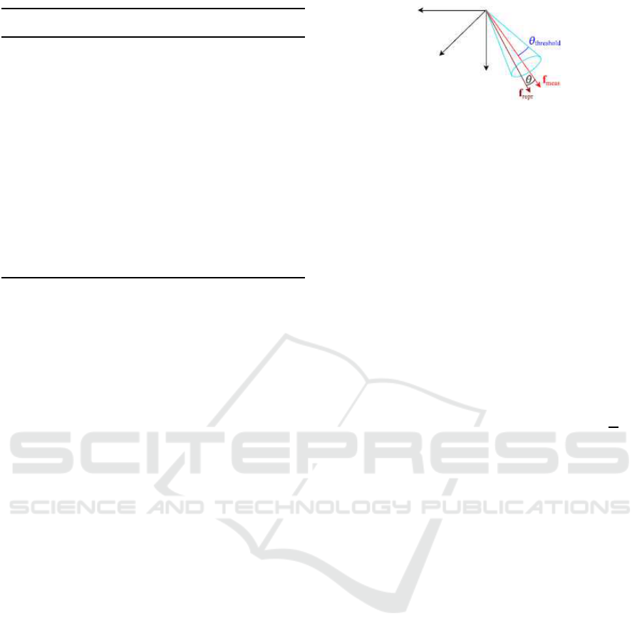
Indeed, the triangulation method used in our im-
plementation follows the general scheme employed in
(Kneip and Furgale, 2014). The reprojection error of
3D bearing vectors was proposed in (Kneip and Fur-
gale, 2014) as well, and is computed by considering
the angle between the measured bearing vector f
meas
and the reprojected one f
repr
. In fact, the scalar prod-
uct of f
meas
and f
repr
directly gives the angle between
them, which is equal to cosθ as illustrated in Figure
3. The reprojection error is, therefore, expressed as
ε = 1− f
T
meas
f
repro
= 1 − cosθ. (8)
Figure 3: Reprojection error computation in Opengv
(Source: (Kneip and Furgale, 2014)).
3.3 RANSAC Rating Kernel
In order to validate each estimated model, we com-
pute a loss value for each datapoint of the dataset. The
loss value is used to verify the model by computing
the reprojection error of all triangulated bearing vec-
tors of the dataset. Outliers are subsequently found
by thresholding the reprojection errors, and the best
model refers to the one with the maximum number of
inliers. As the entire operation is in 3D, we use the
thresholding scheme adopted in the Opengv library
(Kneip and Furgale, 2014). This latter uses a thresh-
old angle θ
threshold
to constrain f
repr
to lie within a
cone of axis f
meas
and of opening angle θ
threshold
as
depicted in Figure 3. The threshold error is given by
ε
threshold
= 1 − cosθ
threshold
= 1 − cos(arctan
ψ
l
),
(9)
where ψ refers to the classical reprojection error
threshold expressed in pixels and l to the focal length.
The model validation process considers multiple
accesses to global memory to evaluate whether each
correspondance of the dataset is an inlier or an out-
lier which is a very execution-time consuming. The
shared memory is, hence, used asa cache to accelerate
computations. The RANSAC rating kernel employs a
block level parallelism and is lauched with iterations
blocks to make each block handles a RANSAC model
and 8 × warpsize threads. Since warpsize = 32, a
total of 256 threads is launched per block and each
thread in the block evaluates a point. To load data-
points in shared memory, a buffer is allocated of size
256 × s where s refers to the size of each datapoint.
In case of bearing vectors, s = 6. Each thread tri-
angulates bearing vector correspondances into a 3D
point and computes its reprojection error according to
Equation 8. This latter is, thereafter, compared to the
precalculated threshold according to Equation 9 to de-
cide whether the correspondance refers to an inlier or
to an outlier. In our implementation, the number of
inliers for 256 values is automatically returned via:
inlier_count=__syncthreads_count(
reproj_error[threadIdx.x]<threshold);
The process of loading data into buffer and
evaluating 256 reprojection errors is repeated
VISAPP 2017 - International Conference on Computer Vision Theory and Applications
112

ceil(datasetCount/256) times.
3.4 RANSAC Best Model Computation
Kernel
This kernel is launched with one block and
itearationsthreads and performs a reduction in shared
memory to derive the best model which refers to the
one with the maximum number of inliers.
4 EVALUATION
In this section we evaluate the speed and accuracy
of our CUDA based essential matrix solver within
RANSAC and compare it against the CPU based im-
plementation for general relative camera motion pro-
vided in the OpenGV library. This latter is an open-
Source library that operates directly in 3D and pro-
vides implementations to solve the problems of com-
puting the absolute or relative pose of a generalized
camera (Kneip and Furgale, 2014).
4.1 Random Problem Generation
To make synthetic data for our tests, we used the au-
tomatic benchmark for relative pose included in the
Matlab interface of the OpenGV library. We used the
provided experiment to create a random relative pose
problem, that is, correspondences of bearing vectors
in two viewpoints using two cameras at the number
of 1000 correspondences. In fact, the number of 1000
correspondences has been chosen based on an aver-
aged number obtained from real images. The experi-
ment returns the observations in both viewpoints (as-
sumed to be a stereo camera system), plus the ground
truth values for the relative transformation parame-
ters.
4.2 Timing
We have measured the mean time while running on
the GPU and CPU (using OpenGV library). To com-
pute the mean time, each estimation is repeated 20
times. The repetition rate is required since a single
estimation can be much slower or much faster than
the mean due to the randomization. We will present
results of computations for both single-precision and
double-precision datatypes. The system on which the
code has been evaluated is equipped with an i7 CPU
running at up to 3.5 GHz, the intel i7 CORE. The
CUDA device is an NVIDIA GeForce GTX 850M
running at 876 MHz with 4096 MB of GDDR5 de-
vice memory. The evaluation has been performed
0 0.1 0.2 0.3 0.4 0.5 0.6 0.7
0
50
100
150
200
250
outlier ratio
mean computation time (ms)
CPU
GPU double precision
GPU single precision
(a) mean time
0 0.1 0.2 0.3 0.4 0.5 0.6 0.7
0
1
2
3
4
5
6
7
8
outlier ratio
mean speedup
GPU single precision
GPU double precision
(b) speedup
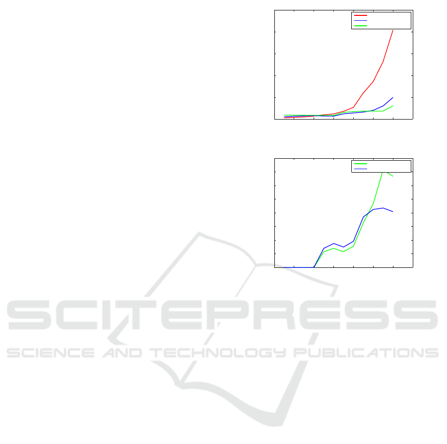
Figure 4: Performance of essential matrix estimation with
RANSAC.
with CUDA version 7.5 integrated with VisualStu-
dio 2012. At the first execution of the estimation,
memory allocations have to be performed. This is re-
quired only once and takes about 6ms. To evaluate
our implementation, 12 outlier ratios from ε = 0.05
to ε = 0.6 in steps of ε = 0.05 are evaluated. In Fig-
ure 4, we show the performance results of estimat-
ing camera relative pose from sets of 2D bearing vec-
tors correspondences. Firstly, in Figure 4a, we com-
pare the mean computation time of CPU and GPU
implementations, in single and double precision. We
show a mean computation time even more important
for CPU reaching 86ms for an outlier ratio ε = 0.5
against 20.2ms for GPU in double precision and 18ms
in single precision. With an outlier ratio of ε = 0.5
which is common for the essential matrix estimation
from automatically computed point correspondences,
we show in figure 4b that the speedup is about 4×
compared to the CPU implementation in single and
double precision. The speedup becomes more im-
portant for higher outlier ratios reaching 7× in single
precision for ε = 0.6 against 4× in double precision.
Furthermore, it is useful to visualize the intersection
between each CPU and GPU evaluation, i.e. the out-
lier ratio where the speedup is equal to one. Figure
4 shows that there is no speedup for lower outlier ra-
CUDA Accelerated Visual Egomotion Estimation for Robotic Navigation
113

tios ε ≤ 0.2. This is because the needed number of
iterations for ε = 0.2 is only 12 iterations. However,
the minimum number of iterations used in GPU based
implementation is 32 iterations referring to the warp
size.
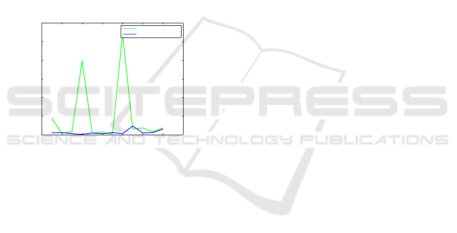
4.3 Accuracy
In Figure 5, we present the Root-mean-square error
(RMSE) between the ground truth rotation matrix and
our Cuda based implementation rotation matrix of the
best model for different outlier ratios, for both single
and double precision datatypes. Overall, single pre-
cision datatype showed good performance while en-
suring higher levels of speedup for higher outlier ra-
tios. The accuracy loss is mostly due to the batched
durand-kerner version for solving 10
th
degree poly-
nomials where the maximum number of iterations is
fixed.
0 0.1 0.2 0.3 0.4 0.5 0.6 0.7
0
1
2
3
4
5
6
x 10
−5
outlier ratio
RMSE error
GPU single precision
GPU double precision
Figure 5: RMSE in rotation between ground truth and
CUDA best model.
5 CONCLUSIONS
In this paper we have presented a 2D-2D robust mo-
tion estimation on CUDA which is applicable to a
wide range of problems and especially to autonomous
navigation. We presented our parallelization strategy,
based mainly on performing the required RANSAC
iterations in parallel. We described our implementa-
tion dealing with several levels of parallelism namely,
warp level parallelism, block level parallelism and
thread level parallelism. In addition, we adapted
the five-point essential matrix using Gr¨obner basis
to CUDA ressources and programming model. Fur-
thermore, we described our RANSAC implementa-
tion and the rating measure used which is based on the
computation of the reprojection error of triangulated
3D points from bearing vectors. An evaluation of
our implementation has been presented and the mean
computation time of RANSAC for different outlier
ratios has been measured. Overall, the implementa-
tion showed good performance, and a speedup 4 times
faster than the CPU was measured for an outlier ratio
ε = 0.5, common for the essential matrix estimation
from automatically computed point correspondences.
More speedup was shown when dealing with higher
outlier ratios.
REFERENCES
Chang, C.-C. and Lin, C.-J. (2011). Libsvm: A library for
support vector machines. volume 2, pages 1–27.
Dissanayake, M. W. M. G., Newman, P., Clark, S., Durrant-
whyte, H. F., and Csorba, M. (2001). A solution to
the simultaneous localization and map building (slam)
problem. In IEEE Transactions on Robotics and Au-
tomation, volume 17, pages 229–241.
Durrant-Whyte, H. and Bailey, T. (2006). Simultaneous lo-
calisation and mapping (slam): Part i the essential al-
gorithms. volume 2, page 2006.
Fischler, M. A. and Bolles, R. C. (1981). Random sample
consensus: A paradigm for model fitting with appli-
cations to image analysis and automated cartography.
volume 24, pages 381–395.
Hartley, R. I. and Zisserman, A. (2004). Multiple View Ge-
ometry in Computer Vision. Cambridge University
Press, ISBN: 0521540518, second edition.
I. Comport, A., Malis, E., and Rives, P. (2010). Real-time
quadrifocal visual odometry. volume 29, pages 245–
266.
Kneip, L. and Furgale, P. (2014). Opengv: A unified and
generalized approach to real-time calibrated geomet-
ric vision.
Li, B., Zhang, X., and Sato, M. (2014). Pitch angle estima-
tion using a vehicle-mounted monocular camera for
range measurement. volume 28, pages 1161–1168.
Lindholm, E., Nickolls, J., Oberman, S., and Montrym, J.
(2008). Nvidia tesla: A unified graphics and comput-
ing architecture. volume 28, pages 39–55.
Maimone, M., Cheng, Y., and Matthies, L. (2007). Two
years of visual odometry on the mars exploration
rovers. volume 24, page 2007.
Nister, D. (2004). An efficient solution to the five-point
relative pose problem. volume 26, pages 756–777.
Nister, D., Naroditsky, O., and Bergen, J. (2006). Visual
odometry for ground vehicle applications. volume 23,
page 2006.
NVIDIA (2015). Cublas documentation.
http://docs.nvidia.com/cuda/cublas/. Online.
Stewenius, D. H., Engels, C., and Nistr, D. D. (2006). Re-
cent developments on direct relative orientation. vol-
ume 60, pages 284–294.
Stewenius, H. and Engels, C. (2008). Mat-
lab code for solving the fivepoint problem.
http://vis.uky.edu/˜stewe/FIVEPOINT/. Online.
Wu, C., Agarwal, S., Curless, B., and Seitz, S. (2011). Mul-
ticore bundle adjustment. pages 3057–3064.
Yonglong, Z., Kuizhi, M., Xiang, J., and Peixiang, D.
(2013). Parallelization and optimization of sift on gpu
using cuda. pages 1351–1358.
VISAPP 2017 - International Conference on Computer Vision Theory and Applications
114