Pose Interpolation for Rolling Shutter Cameras using Non Uniformly

Time-Sampled B-splines

Bertrand Vandeportaele

, Philippe-Antoine Gohard

1,2

, Michel Devy

and Benjamin Coudrin

LAAS-CNRS, Universit

e de Toulouse, CNRS, UPS, Toulouse, France

Innersense, Ramonville-Saint-Agne, France

{bertrand.vandeportaele, philippe-antoine.gohard, michel.devy}@laas.fr, benjamin.coudrin@innersense.fr

Keywords:

Rolling Shutter, Camera Geometric Model, Perspective n-Points Algorithm, Simultaneous Localization and

Mapping, B-splines interpolation.

Abstract:

Rolling Shutter (RS) cameras are predominant in the tablet and smartphone market due to their low cost and

small size. However, these cameras require speciﬁc geometric models when either the camera or the scene is

in motion to account for the sequential exposure of the different lines of the image. This paper proposes to

improve a state-of-the-art model for RS cameras through the use of Non Uniformly Time-Sampled B-splines.

This allows to interpolate the pose of the camera taking into account the varying dynamic of the motion by

adding more control points where needed while keeping a low number of control points where the motion is

smooth. Two methods are proposed to determine adequate distributions for the control points, using either an

IMU sensor or an iterative reprojection error minimization. Results on simple synthetic data sets are shown to

prove the concept and future works are introduced that should lead to the integration of our model in a SLAM

algorithm.

1 INTRODUCTION

In Augmented Reality applications for mobile devices

(smartphones and tablets), the realtime localization of

the device camera and the 3D modeling of the envi-

ronment are used to integrate virtual elements onto

the images of the real environment. This task is

usually performed by algorithms of Structure From

Motion (SFM: (Hartley and Zisserman, 2004)), and

Simultaneaous Localization and Mapping (SLAM:

MonoSLAM(Davison, 2003), PTAM(Klein and Mur-

ray, 2007) OrbSLAM (Mur-Artal et al., 2015)). Most

existing implementations assume that the cameras are

using a Global Shutter (GS), for which all the lines of

the image are exposed at the same time, ie. the image

is a projection of the scene at one instant t.

However, more than 90% of mobile devices are

equipped with Rolling Shutter (RS) cameras because

of their lower cost and smaller size than the classic GS

cameras. The advantages of RS cameras come with

some drawbacks; by the way they are designed, they

cause image distortions when observing a dynamic

scene or when the camera is moving. In these sensors,

all the lines of the image are exposed and transferred

sequentially at different times.

More complex geometric models are thus required

for RS cameras, to account for the the varying pose of

the camera. This paper extends the RS Camera model

presented in(Steven Lovegrove, 2013) and (Patron-

Perez et al., 2015) for the camera pose interpolation

using B-splines controlled by Control Points (CP) that

are Uniformly Distributed (UD) in time. Our im-

provement of the model consists in using an adaptive

Non Uniform Distribution (NUD) of the CP of the B-

spline over time. This allows to globally reduce the

number of CP required to model a given trajectory

with the same accuracy than using UD.

The paper ﬁrstly presents existing SLAM algo-

rithms and exhibits problems arising from using im-

ages captured with RS cameras. It then presents the

theoretical framework used for the modeling of the

RS cameras. First, the cumulative B-splines are in-

troduced to allow the interpolation of 6-dof camera

pose in continuous time. Second, the pinhole camera

model using interpolated poses is derived. Finally,

the iterative minimization used in the Perspective n-

Points algorithm is explained. Our contribution fo-

cused on the distribution of the CP is then studied

and two methods are proposed to determine adequate

NUD of the CP, using either information from an IMU

sensor or multiple iterations of reprojection error min-

imization. The two methods are evaluated on sim-

286

Vandeportaele B., Gohard P., Devy M. and Coudrin B.

Pose Interpolation for Rolling Shutter Cameras using Non Uniformly Time-Sampled B-splines.

DOI: 10.5220/0006171802860293

In Proceedings of the 12th International Joint Conference on Computer Vision, Imaging and Computer Graphics Theory and Applications (VISIGRAPP 2017), pages 286-293

ISBN: 978-989-758-227-1

ple synthetic data sets to prove the concept and future

works are introduced that should lead to the integra-

tion of our model in a SLAM algorithm.

2 RELATED WORK FOR SLAM

2.1 Global Shutter

A SLAM algorithm can recover the position and ori-

entation of a mobile camera. In the Augmented Re-

ality context, these camera parameters can be used

to synthesize images of virtual elements as if they

were seen by the real camera. To do so without prior

knowledge of the environment, it is necessary to map

it in realtime.

Early realtime methods used to solve the SLAM

problem in the literature were based on Extended

Kalman Filter (EKF)(Davison, 2003), (Roussillon

et al., 2012), (Gonzalez, 2013). The simplicity of this

method and it’s computing efﬁciency for small size

environment model has made it the most used SLAM

method for the past decade.

Other robust and realtime methods based on lo-

cal Bundle Adjustment like PTAM (Klein and Mur-

ray, 2007) have also been proposed. They minimize

the reprojection error over a subset of previously ac-

quired images, called keyframes (Engel et al., 2014),

(Mur-Artal et al., 2015), or over a sliding window of

frames (Mouragnon et al., 2006). They provide im-

proved robustness thanks to the modeling of outliers,

and (Strasdat et al., 2010) proved the superiority of

these Bundle Adjustment-based methods over ﬁlter-

ing one.

2.2 Rolling Shutter

Using a SLAM method designed for GS camera

model with RS camera produces deviations of the es-

timated trajectory and reconstructed 3D points. These

deviations increase with the velocity of the cam-

era. One of the ﬁrst use of a RS camera model

in the SLAM context was the adaptation of PTAM

for smartphone (Klein and Murray, 2009). They es-

timated the angular velocity of the camera at the

keyframe using keypoints tracked between the previ-

ous and the next frame. This angular velocity was

then used to correct the measurements of the points

in the image using a ﬁrst order approximation so they

can be used as if they where obtained by a GS camera.

(Hedborg et al., 2011) initially used a similar

method, and proposed in (Hedborg et al., 2012) a bun-

dle adjustment using a RS camera model. To estimate

the varying camera pose inside a frame, they interpo-

lated independently the rotations (using SLERP) and

the translations (using linear interpolation).

(Furgale et al., 2012) also used a system based on

B-splines to have a continuous time representation. In

their work, they interpolate rotations and translations

by two independent B-splines. Their Cayley-Gibbs-

Rodriguez formulation used for the poses had two ma-

jor issues according to (Steven Lovegrove, 2013):

• The used Rodrigues parameterization has a singu-

larity for the rotation at π radians.

• The interpolation in this space does not repre-

sent the minimum distance for the rotation group

hence the generated trajectories can correspond to

unrealistic motions.

To address these issues,(Steven Lovegrove, 2013)

proposed to use a continuous time trajectory formu-

lation using cumulative B-splines. Their theoretical

framework is the basis of our work and is derived

next.

3 THEORETICAL FRAMEWORK

FOR RS CAMERAS

3.1 Cumulative B-splines for Pose

Interpolation

A standard B-spline is deﬁned by constant polynomial

basis functions B

i,k

(k −1 being the degree of the used

polynomial) and variable Control Points (CP) p

p(t) =

k−1

∑

i=0

i,k

(t) (1)

Let

i,k

(t) =

∑

k−1

j=i

j,k

(t) be a cumulative basis func-

tions deﬁned further in eq. (8). The eq. (1) can be re-

formulated using CP differences (p

− p

i−1

) to obtain

the cumulative B-splines expression:

p(t) = p

0,k

(t)+

k−1

∑

i=1

− p

i−1

)

i,k

(t) (2)

This deﬁnition of the B-spline stands for multidi-

mensional spaces and thus allows the interpolation for

camera poses p(i) ∈ R

independently over its differ-

ent components (for instance 3 translation parameters

and 3 rotation parameters using Rodrigues parame-

terization). However this does not account for the

correlations between the components of the pose thus

some adaptations are required to overcome this, using

6DoF camera poses deﬁned in the SE3 space. Such

poses can be expressed by transformation matrices T

Pose Interpolation for Rolling Shutter Cameras using Non Uniformly Time-Sampled B-splines

287

parameterized by a translation a and a rotation matrix

T =



R a



,T ∈ SE3,R ∈ SO3,a ∈ R

(3)

While the cumulative B-splines interpolation in

involves the differentiation of CP (p

− p

i−1

), in

the special Euclidean group SE3 it requires more

complex operations. Let T

w,i

be the i

Control Poses

(indistinctly abbreviated as CP) relatively to the world

coordinate frame w, the transformation matrix ∆T

i−1,i

relating two poses T

w,i−1

and T

w,i

is obtained by com-

position:

∆T

i−1,i

= T

−1

w,i−1

w,i

(4)

The log function maps a pose (or variation) deﬁned

in SE3 to its tangent space se3, where operations for

composing transformation are simpler, and allows to

express the summation of weighted CP variation by

simple addition. Let T

w,s

(t) be the interpolated pose

along the B-spline at instant t and ∆

be the time be-

tween the 2 poses. Let Ω

i−1,i

∆

log(∆T

i−1,i

), the

eq. (2) can be adapted to se3:

log(T

w,s

(t)) =

(t)log(T

w,0

) +

k−1

∑

i=1

(t)Ω

i−1,i

(5)

The inverse of the logarithmic map, the exponen-

tial map, projects a pose from se3 to SE3 and can

be used to recover T

w,s

(t)) = exp(log(T

w,s

(t))). Ob-

serving that additions in se3 maps to multiplications

in SE3, the eq.(5) can be reformulated for SE3. The

pose T

w,s

(t) (for the B-spline s and expressed in world

coordinates w) is interpolated between the two CP

w,i

and T

w,i+1

for different time t using :

w,s

(t) = exp(

(t)log(T

w,0

))

k−1

∏

i=1

exp(

(t)Ω

i−1,i

)

(6)

A change of variable is introduced to map the real

time t variable between two CP associated to times

and t

+ ∆

to a normalized time u ∈ [0, 1] interval,

using a constant time interval ∆

between the CP:

u = (t −t

)/∆

(7)

Using this normalized time, the time between 2 CP is

equal to one, so the factor

∆

vanishes and the ex-

pression of Ω

i−1,i

can be reformulated as Ω

i−1,i

log(∆T

i−1,i

)

(Steven Lovegrove, 2013) have chosen to use cu-

bic B-splines because of their C

continuity, which

allow to predict angular velocities and linear acceler-

ations. Hence the degree of the polynomial for the

basis is 3 and the B-splines are locally controlled by

4 CP (as k = 4), meaning that the knowledge of the 4

surrounding CP is sufﬁcient to interpolate on the B-

spline. The used cumulative basis functions

i,k

(u)

for k = 4 are expressed in the i

component of the

vector

B(u) by:

B(u) =







6 0 0 0

5 3 −3 1

1 3 3 −2

0 0 0 1



















(8)

Using normalized time variable u and noting that

the ﬁrst line of

B(u) is

(u) = 1, the eq.( 6) can be

simpliﬁed in:

w,s

(u) = T

w,0

k−1

∏

i=1

exp(

(u)Ω

i−1,i

) (9)

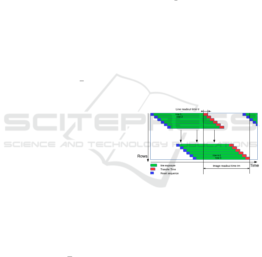
3.2 Rolling Shutter Camera Model

An image from a RS camera can be seen as the con-

catenation of one dimensional images (rows) exposed

at different times as seen in the ﬁgure 1.

Figure 1: RS cameras expose the image lines sequentially,

thus if the ﬁrst line is exposed at instant t

, then the n

line

is exposed at t

+ n.t

with t

the readout time of a line. The

time taken by the camera to fully expose an image is called

the readout time t

. (Li et al., 2013).

For a static scene and camera, there is no geomet-

ric difference between the GS and RS camera. But if

the camera is in motion relatively to the scene, each

line is a projection from a different camera viewpoint.

While the camera pose T ∈ SE3 is common to all the

pixels in a GS image, it varies over time as T(t) for

each individual line in the RS case.

The pinhole camera perspective projection model

is derived below. Let X be a 3D point deﬁned in ho-

mogeneous coordinates in the world coordinate sys-

tem w. Let T

w,c

be the transformation matrix from

world w to camera c coordinate frame. Let K be the

camera matrix containing the intrinsic parameters and

π(.) be the perspective projection (mapping from P

VISAPP 2017 - International Conference on Computer Vision Theory and Applications

288

to R

). The pinhole model projects X onto the image

plane to



x y



by:





:= π([K|0]T

w,c

X) (10)

To model the varying pose over time T

w,c

is pa-

rameterized by t as T

w,c

(t). The spline being deﬁned

by eq.( 9) in the spline coordinate frame s (attached

to the IMU for instance) different from c, a (constant

over time) transformation T

s,c

is required to obtain

w,c

(t):

w,c

(t) = T

s,c

w,s

(t) (11)

The projection at varying time t is obtained by:



x(t)

y(t)



:= π([K|0]T

w,c

(t)X) = ω(X,T

w,c

(t)) (12)

This model does not yet represent the fact that at a

given time t corresponds a single line exposure. So

the projection



x(t

) y(t

)



of X at time t = t

will

actually be obtained only if the line y(t

) is exposed

at time t

(Steven Lovegrove, 2013) expressed the line ex-

posed at a time t as a function of s the frame start

time, e is the end frame time, and h is the height of

the image in pixels by:

y(t) = h

(t − s)

(e − s)

(13)

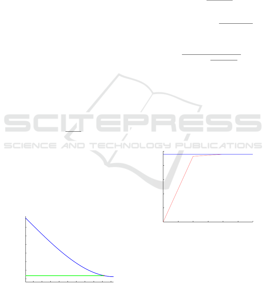
The ﬁgure 2 shows plotted in blue the image pro-

jections



x(t) y(t)



of a single 3D point obtained

by eq.( 12) using interpolation of the poses deﬁned in

eq.( 9). The value of t is sampled to the different ex-

posure time of each individual row. The green line in-

dicates the row that is actually exposed when the y(t)

corresponds to the row number and the red cross at

the intersection is the resulting projection. For highly

curved trajectories, multiple projections of a single

3D point can be observed in a single image.

566 568 570 572 574 576 578 580 582 584

414

416

418

420

422

424

426

428

column

rows

Figure 2: Here is an example of the different projections of

a 3D point (in blue) in one image for each of the line poses,

in the case of a moving camera. The green line shows the

exposed rows at the time the 3D point is projected to it.

The projection(s)



x(t) y(t)



that is(are) effec-

tively observed by the RS camera is(are) obtained by

intersecting the curves corresponding to eq.( 12) and

eq.( 13). Determining t is an optimization problem

that (Steven Lovegrove, 2013) solve iteratively using

ﬁrst order Taylor expansion of the 2 equations around

a time t:

(t + δt) = h

(t + δt − s)

(e − s)

(14)



x(t + δt)

y(t + δt)



= ω(X , T

w,c

(t))+ δt

dω(X,T

w,c

(t))

(15)

This system of equations is reorganized as:

δt = −

ht + s(y

(t)− h) − ey

(t)

h + (s −e)

dω

(X,T

w,c

(t))

(16)

By updating t as t = t + δ

and iterating, t con-

verges generally in approximately 3 or 4 iterations

(see Figure 3). Once t is determined, the correspond-

ing projection is obtained using eq.( 12). For slow

motions, the initial value for t can be set at the time

corresponding to the middle row of the image and the

iterative algorithm is very likely to converge. How-

ever, for high dynamic motions, the initial value has

to be set wisely, as different initial values could lead

to different projections that correspond indeed to dif-

ferent actual projections.

0 0.5 1 1.5 2 2.5 3

2.35

2.4

2.45

2.5

2.55

2.6

iteration number

Figure 3: Evolution of t during three iterations.

3.3 Perspective n-Points Algorithm for

RS Camera

The Perspective n-Points, or PnP algorithm consists

in determining the pose of a camera given n corre-

spondences between 3D known points and their ob-

servations in the image. Here we describe the itera-

tive portion of the PnP algorithm that is used to reﬁne

a ﬁrst estimate.

Pose Interpolation for Rolling Shutter Cameras using Non Uniformly Time-Sampled B-splines

289

Let u

i,k

be a set of image measurements (corre-

sponding to time t

) of M 3D points X

inside a set

of N images and T

w,c

be related to a set of CP T

w,s

through eq.( 11).The reprojection error res(i,k) for in-

dividual point is deﬁned by:

res(i,k) = ||u

i,k

− π([K|0]T

w,c

)|| (17)

The following cost function is minimized to de-

termine

θ, the set of parameters T

w,s

that best ﬁts the

model to the set of observations:

θ = argmin

∑

i=1

∑

k=1

res(i,k)

(18)

While a PnP algorithm for a GS camera optimizes

the pose of the camera itself, the RS version has to

optimize the CP used for the interpolation. Thus, the

parameters vector θ contains the required CP param-

eters.

The minimization is achieved using the

Levenberg-Marquardt algorithm, an iterative non-

linear least squares solver behaving between

Gauss-Newton and Gradient Descent. The initial

value for the parameters in θ is set from the IMU

measurements or by applying ﬁrstly a GS PnP.

The levenberg Marquardt algorithm uses the partial

derivatives (obtained by ﬁnite difference) of the cost

function with respect to the parameters to optimize.

It generally converges after several iterations but

is prone to converge to local minimum if the cost

function is not convex or if the initial value is too far

from the global minimum.

4 CP TEMPORAL SAMPLING

4.1 Uniform Distribution

(Steven Lovegrove, 2013) use an UD in time for

the CP, and use normalized times as shown in

eq.( 7). This UD of CP (chosen every 0.1 seconds in

(Steven Lovegrove, 2013)) leads to some limitations

in these two cases:

• For a camera grabbing frames at 30FPS, a CP

is deﬁned each 3 frames leading to relatively

smoothed trajectory for fast camera motions, fail-

ing to accurately model it.

• For steady movement, the algorithm creates un-

necessary redundant CP.

The motion of hand-held device used for aug-

mented reality can be decomposed in three distinct

type of motions: high speed motion, low speed mo-

tion, and low range but high frequency motions when

the user’s hand is shaking. While the use of a small

UD interval ∆

between CP is a a simple solution to

model theses motions, it leads to an increase of the CP

number and consequently of the computational cost.

Doing so, unnecessary CP are used for low speed and

steady motions, adding no information/constraints to

the interpolated trajectory.

4.2 Non Uniform Distribution

To overcome this problem, we propose to relax the

UD constraint for the intervals ∆

between the CP.

This allows to locally increase the number of CP

where needed by lowering the time interval ∆

dur-

ing fast motion while keeping a low number of CP

for portions of the trajectory that correspond to slow

motions.

The mapping between u and t is then deﬁned dif-

ferently from eq.( 7) by:

u =

t −t

i+1

−t

(19)

While the retrieving of the t

and t

+1 CP involved

only multiplication and rounding in the UD case, it re-

quires more complex computations with NUD as the

time value t

can be deﬁned freely.

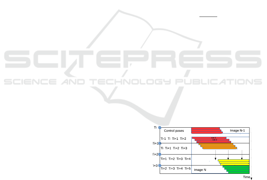
NUD provides the ability to create locally multi-

ple CP inside a single image. This leads to many CP

quartets required to interpolate the pose inside differ-

ent portions of the image (see Figure 4). As retrieving

the CP associated to a time t is an operation that is

done thousands of times per frame, some care is re-

quired to avoid wasting time searching over all the CP.

This is achieved by storing CP indices in an chrono-

logically ordered list and using hash tables for fast

access.

Figure 4: An example of multiple CP inside a single image,

and their inﬂuence for interpolating the pose for different

rows. 3 CP are time-stamped between the beginning and

the end of the image N: T

i+1

, T

i+2

and T

i+3

. The quartet

of CP used for interpolating pose at each row change three

time during the image exposure.

VISAPP 2017 - International Conference on Computer Vision Theory and Applications

290

4.3 CP Generation Methods

As our approach uses varying time intervals function

of the local properties of the motion, it requires to

generate the CP at the right time. We investigated two

different approaches involving either an IMU sensor

or the analysis of the reprojection error in the images.

The ﬁrst one is better ﬁtted for realtime applications

as the CP can be generated online using IMU mea-

surements while the second involves an iterative pro-

cess that predisposes it for ofﬂine computation.

4.3.1 Based on IMU

An IMU sensor is generally composed of a gyroscope

that measures the angular velocities and accelerom-

eters that provide accelerations. On current tablets

and smartphones, it generally delivers measurements

at about 100Hz, which is an higher frequency than the

frame rate of the camera.

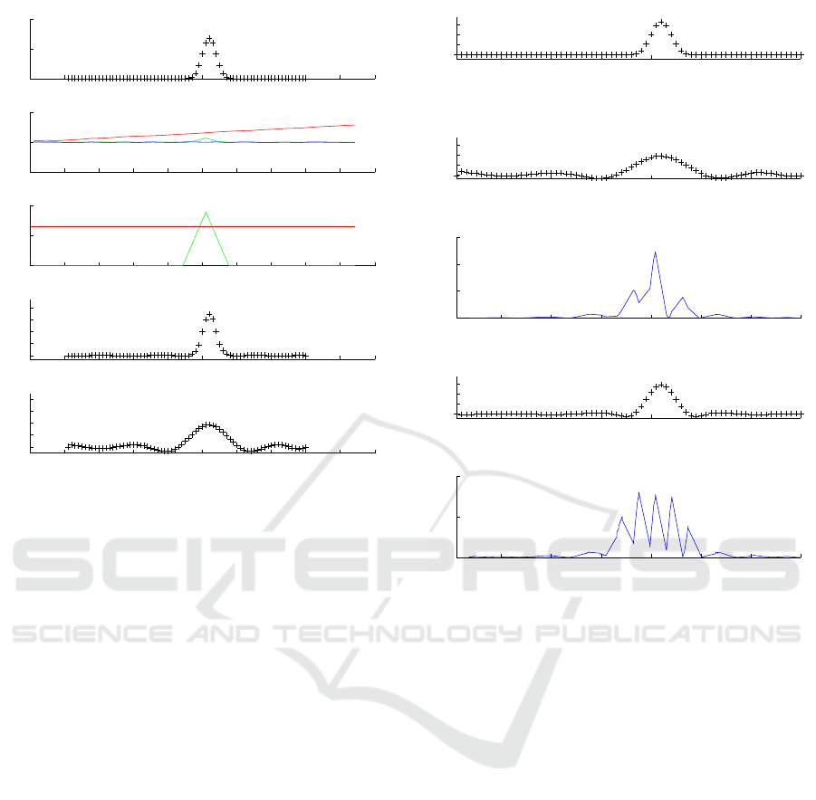
We propose a simple analysis of the measurements

done by the IMU to determine when the CP are re-

quired. The ﬁgure 5 shows a generated trajectory

(in the two top plots). The left (resp. right) plots

corresponds to the translation (resp rotation) compo-

nents. The data provided by the IMU are plotted in

the middle plots. The bottom plots show respectively

the norm of the linear accelerations and angular ve-

locities. Different thresholding values (shown in red,

blue and black) are used to determine when more CP

are required. These threshold values th

are stored in

two (for acceleration and angular velocity) look up

table providing n(th

), the number of CP required per

unit of time. These lists of threshold values are gen-

erated empirically for the moment and correspond to

a tradeoff between accuracy of the motion modeling

and computational cost. For instance, if the angular

velocity norm is below the threshold th

, n(th

) CP

per unit of time are used while if its norm rises above

but below th

, n(th

) CP per unit of time are used

and so on. Once the CP are created, their parameters

are optimized using eq.( 18).

4.3.2 Based on Reprojection Error

We propose a second method to determine the tem-

poral location of the CP when a IMU in not avail-

able. This method involves an iterative estimation of

the trajectory using initial CP (set for instance with

an UD) as shown in eq.( 18). Let res

,∆

be the mean

of the residuals res(i,k) deﬁned in eq.( 17) between

times t

and t

+ ∆

. Our method use an iterative

scheme consisting of the following two steps:

• The residuals are computed along the trajectory

and analyzed using a sliding window to measure

0 0.5 1

−0.2

0.2

Translation

0 0.5 1

−0.5

0.5

Orientation

0 0.5 1

−100

100

Acceleration

0 0.5 1

−4

−2

Angular Velocity

0 0.5 1

100

200

Acceleration norm

0 0.5 1

Angular velocity norm

Figure 5: Determination of the number of required CP per

unit of time using IMU measurements analysis (See the text

for details).

locally res

,∆

for varying t

. Maximums values

are detected and additional CP are generated at

the middle of the two corresponding neighboring

CP for time t

∆

• An iterative estimation of the trajectory eq.( 18)

is achieved with the added CP to reﬁne the whole

set of CP.

The process is iterated until ∀t

: res

,∆

< threshold.

5 RESULTS

We evaluated our methods on simulated data sets con-

sisting of simple scenes (deﬁned by sparse points

clouds) and trajectories (deﬁned by B-splines using

manually deﬁned ground truth CP that are NUD).

While the proposed methods have been tested to

model complex 6-dof trajectories, they cannot be eas-

ily drawn in this paper. Hence the plotted results are

for simple trajectories to allow the reader to interpret

them in 2D and serve as proof of concept. The syn-

thetic scene is projected to synthetic images using the

RS camera model, and the CP are optimized using

the iterative minimization. Even if the plotted results

only show the trajectories, they are computed using

the whole framework presented above ie. using the

PnP algorithm to compare the poses through the re-

projection error in the images using the RS camera

model.

5.1 Based on IMU

To test IMU-based CP generation, IMU measure-

ments are synthesized at 100Hz from the ground truth

trajectory using the ﬁrst and second derivatives of

Pose Interpolation for Rolling Shutter Cameras using Non Uniformly Time-Sampled B-splines

291

0 0.1 0.2 0.3 0.4 0.5 0.6 0.7 0.8 0.9 1

−0.5

0.5

0 0.1 0.2 0.3 0.4 0.5 0.6 0.7 0.8 0.9 1

100

200

0 0.1 0.2 0.3 0.4 0.5 0.6 0.7 0.8 0.9 1

0.05

0.1

0 0.1 0.2 0.3 0.4 0.5 0.6 0.7 0.8 0.9 1

0.02

0.04

0.06

0.08

0 0.1 0.2 0.3 0.4 0.5 0.6 0.7 0.8 0.9 1

0.02

0.04

0.06

0.08

Figure 6: Results for the IMU method (see text for details).

eq.( 6) (see (Steven Lovegrove, 2013) for details).

We set the ﬁrst thresholds for the angular velocity

to th

Rot = 2rad/s and for the linear acceleration to

cc = 130cm/s

The ﬁgure 6 (a) shows a simple trajectory con-

sisting of a linear motion with a perturbation at t=0.5.

The plot 6 (b) shows the position of the camera during

the motion (using different colors for different axes,

the green being used for the vertical direction). The

plot 6 (c) shows the norm of the acceleration in green

while the ﬁrst threshold is plotted in red. The angu-

lar velocities are not plotted in this simple example as

they have null values. The plot 6 (d) shows the B-

spline trajectory generated by our method while 6 (e)

shows the B-spline generated with the same number

of CP but using an UD. As expected, the NUD B-

spline is much closer to the ground truth while the

UD B-spline artiﬁcially smooths the trajectory, and

creates larger oscillations.

5.2 Based on Reprojection Error

For this second test, the same trajectory is used as

shown in ﬁgure 7 (a), but the synthetic IMU measure-

ments are not exploited. A ﬁrst UD for the CP is used

to initiate the process and the resulting B-spline af-

ter one reprojection error minimization step is shown

in (b). The residuals mean value for the sliding win-

dows are shown in (c), and the maximum detected at

t = 0.5 permits to add a few (2) CP in the neighbor-

0.2 0.3 0.4 0.5 0.6 0.7 0.8

0.02

0.04

0.06

0.2 0.3 0.4 0.5 0.6 0.7 0.8

0.02

0.04

0.06

0.2 0.3 0.4 0.5 0.6 0.7 0.8

0.02

0.04

0.06

0.2 0.3 0.4 0.5 0.6 0.7 0.8

Figure 7: Results for the reprojection error method (see text

for details).

hood and iterate with error minimization step. The

process is stopped once the number of CP reaches the

same value than in the plot 6 (d) and (e) for com-

parison purpose. The obtained B-spline trajectory is

shown in 7 (d) and the corresponding residuals mean

value for the sliding windows in (e) shows a decrease

by an approximate 20X factor compared to (c) for a

increase of only 2 CP.

6 FUTURE WORKS

Our future researches will focus on multiple points:

• Some tests on real motions using hand held de-

vices will be conducted, the ground truth being

provided by a motion capture system.

• We will attempt to intricate in the same optimiza-

tion process the minimization of the residuals and

the CP generation in order to lower the time re-

quirements, especially for the method based on

reprojection error.

• Whereas the time associated to the CP are ﬁxed

in our current study, it would be interesting to

VISAPP 2017 - International Conference on Computer Vision Theory and Applications

292

optimize their values alongside the pose param-

eters. This added degree of freedom would allow

to adapt dynamically the distribution in time of

the CP avoiding the generation of new ones.

• We will try to integrate our model in a realtime

SLAM.

7 CONCLUSION

In this paper, we have enriched the B-splines trajec-

tory model from (Steven Lovegrove, 2013) to inte-

grate NUD for the CP in the RS Camera SLAM con-

text. We have shown that this NUD allowed to bet-

ter model trajectories than using an UD for the same

number of CP. We have proposed two methods to

generate the CP, using either IMU measurements or

iterative reprojection error minimization. The two

methods have been tested on synthetic trajectories and

proven to be efﬁcient for the PnP problem resolution.

This enriched model will be integrated in a SLAM in

future works.

REFERENCES

Davison, A. J. (2003). Real-time simultaneous locali-

sation and mapping with a single camera. In 9th

IEEE International Conference on Computer Vision

(ICCV 2003), 14-17 October 2003, Nice, France,

pages 1403–1410.

Engel, J., Sch

ops, T., and Cremers, D. (2014). LSD-SLAM:

Large-scale direct monocular SLAM. In ECCV.

Furgale, P., Barfoot, T. D., and Sibley, G. (2012).

Continuous-time batch estimation using temporal ba-

sis functions. In Robotics and Automation (ICRA),

2012 IEEE International Conference on, pages 2088–

2095.

Gonzalez, A. (2013). Localisation par vision multi-

spectrale. Application aux syst

emes embarqu

es. The-

ses, INSA de Toulouse.

Hartley, R. I. and Zisserman, A. (2004). Multiple View Ge-

ometry in Computer Vision. Cambridge University

Press, ISBN: 0521540518, second edition.

Hedborg, J., Forss

en, P. E., Felsberg, M., and Ringaby, E.

(2012). Rolling shutter bundle adjustment. In Com-

puter Vision and Pattern Recognition (CVPR), 2012

IEEE Conference on, pages 1434–1441.

Hedborg, J., Ringaby, E., Forss

en, P. E., and Felsberg, M.

(2011). Structure and motion estimation from rolling

shutter video. In Computer Vision Workshops (ICCV

Workshops), 2011 IEEE International Conference on,

pages 17–23.

Klein, G. and Murray, D. (2007). Parallel tracking and

mapping for small AR workspaces. In Proc. Sixth

IEEE and ACM International Symposium on Mixed

and Augmented Reality (ISMAR’07), Nara, Japan.

Klein, G. and Murray, D. (2009). Parallel tracking and map-

ping on a camera phone. In Proc. Eigth IEEE and

ACM International Symposium on Mixed and Aug-

mented Reality (ISMAR’09), Orlando.

Li, M., Kim, B., and Mourikis, A. I. (2013). Real-time mo-

tion estimation on a cellphone using inertial sensing

and a rolling-shutter camera. In Proceedings of the

IEEE International Conference on Robotics and Au-

tomation, pages 4697–4704, Karlsruhe, Germany.

Mouragnon, E., Lhuillier, M., Dhome, M., Dekeyser, F.,

and Sayd, P. (2006). Real time localization and 3d

reconstruction. In 2006 IEEE Computer Society Con-

ference on Computer Vision and Pattern Recognition

(CVPR’06), volume 1, pages 363–370.

Mur-Artal, R., Montiel, J. M. M., and Tard

os, J. D. (2015).

Orb-slam: A versatile and accurate monocular slam

system. IEEE Transactions on Robotics, 31(5):1147–

1163.

Patron-Perez, A., Lovegrove, S., and Sibley, G. (2015). A

spline-based trajectory representation for sensor fu-

sion and rolling shutter cameras. Int. J. Comput. Vi-

sion, 113(3):208–219.

Roussillon, C., Gonzalez, A., Sol

a, J., Codol, J., Mansard,

N., Lacroix, S., and Devy, M. (2012). RT-SLAM: A

generic and real-time visual SLAM implementation.

CoRR, abs/1201.5450.

Steven Lovegrove, Alonso Patron-Perez, G. S. (2013).

Spline fusion: A continuous-time representation for

visual-inertial fusion with application to rolling shut-

ter cameras. In Proceedings of the British Machine

Vision Conference. BMVA Press.

Strasdat, H., Montiel, J., and Davison, A. J. (2010). Real-

time monocular slam: Why ﬁlter? In Robotics and

Automation (ICRA), 2010 IEEE International Confer-

ence on, pages 2657–2664. IEEE.

Pose Interpolation for Rolling Shutter Cameras using Non Uniformly Time-Sampled B-splines

293