Online Eye Status Detection in the Wild with Convolutional Neural
Networks
Essa R. Anas, Pedro Henriquez and Bogdan J. Matuszewski
Computer Vision and Machine Learning Research Group,
School of Engineering, University of Central Lancashire, Preston, U.K.
Keywords: Convolutional Neural Network CNN, Deep Learning, Eye Status Detection, Eye Blinking Estimation.
Abstract: A novel eye status detection method is proposed. Contrary to the most of the previous methods, this new
method is not based on an explicit eye appearance model. Instead, the detection is based on a deep learning
methodology, where the discriminant function is learned from a large set of exemplar images of eyes at
different state, appearance, and 3D position. The technique is based on the Convolutional Neural Network
(CNN) architecture. To assess the performance of the proposed method, it has been tested against two
techniques, namely: SVM with SURF Bag of Features and Adaboost with HOG and LBP features. It has been
shown that the proposed method outperforms these with a considerable margin on a two-class problem, with
the two classes defined as “opened” and “closed”. Subsequently the CNN architecture was further optimised
on a three-class problem with “opened”, “closed”, and “partially-opened” classes. It has been demonstrated
that it is possible to implement a real-time eye status detection working with a large variability of head poses,
appearances and illumination conditions. Additionally, it has been shown that an eye blinking estimation
based on the proposed technique is at least comparable with the current state-of-the-art on standard eye
blinking datasets.
1 INTRODUCTION
The recent interest in the eye status and blinking
detection is reflected by a large number of new
publications related to numerous relevant
applications. For instance, driver assistance systems
use eye tracking and eye status detection to assess
driver attentiveness (Du et al., 2008). In psychology,
the frequency of the blinking is used to estimate stress
while attending a job interview (Marcos-Ramiro et
al., 2014), or fatigue detection of students (Joshi et al.,
2016) during an online learning. In (Wascher et al.,
2015) authors correlated the awareness of the subject
to the new information by measuring the blinking
rate. The eye status detection was also utilized in
assisting the human interaction (Królak et al., 2012),
(Mohammed et al., 2014). The objective, in these
studies, was helping people with special needs in
controlling the execution of common tasks using their
eyes. The eye status detection has been also used to
assess the eye health. In that case, changes in an
average estimated number of blinks are linked to a
specific eye condition (Sun et al., 2013). In case of
eye dryness the number of blinks is expected to
increase (Divjak and Bischof, 2009). Similarly, it has
been reported that computer users’ blinking rate
decreases to 60% compared to the normal blinking
rate of 10-15 times a minute (Fogelton and Benesova,
2016). Blinking detection can be also used against
spoofing in face recognition systems (Pan et al.,
2007) (Szwoch et al., 2012).
The eye blink is defined by changes in the eye
status between opened, partially-opened, and closed.
A so called complete blink occurs when the eye status
is changing sequentially between the three states
within a specified timeframe, typically between 100
and 400 milliseconds. The incomplete and extended
blinks are also defined, and happen respectively,
when either the closed state is not completely
reached, or it takes longer to execute (Portello et al.,
2013). A number of methods have been proposed for
the blink detection. They are either based on
identifying the eye state in each individual frame, and
subsequently combining the outcomes, or by
detecting the motion of the eyelids by processing
multiple image frames at once.
88
Anas E., Henriquez P. and Matuszewski B.
Online Eye Status Detection in the Wild with Convolutional Neural Networks.
DOI: 10.5220/0006172700880095
In Proceedings of the 12th International Joint Conference on Computer Vision, Imaging and Computer Graphics Theory and Applications (VISIGRAPP 2017), pages 88-95
ISBN: 978-989-758-227-1
Copyright
c
 2017 by SCITEPRESS – Science and Technology Publications, Lda. All rights reserved

2 RELATED WORK
The most frequent approach for eye status and
blinking estimation uses face and eyes area detections
as a pre-processing step. The Viola-Jones (Viola and
Polatsek, 2004) method is the most common
technique applied for relevant area detection. This is
sometimes followed by face/eye tracking to handle
the out-of-plane (Saragih et al., 2011) and/or in-plane
head rotations (Tomasi and Kanade, 1991)
The eye status detection is often the first stage to
estimate the blinking rate as in Du et al., 2008. After
detecting the face and eye areas, the cropped eye
images are binarized and resized to 12x30 pixels. The
estimate is based on the ratio of the length of the
detected eye to its width, with an empirically set
threshold. The authors reported 91.16% accuracy
using this technique. However the dataset used for
comparison was not provided.
Similarly, Lee et al., 2010 extract two features that
describe the eye status, open or close. To have a
meaningful estimation, illumination normalization is
performed first and subsequently the eye images are
binarized. The Support Vector Machine (SVM) is
used as a classifier operating on features derived from
the binary images. The method showed a recall of
92% on the ZJU dataset (Pan et al., 2007).
A specific geometry of the eye can also be applied
to extract features that can be used to train a Neural
Network (NN) to estimate the eye status and
consequently the blinking. Danisman et al., 2010,
suggested using the pupil to detect the eye status. If
the eye is open, then the upper half of the pupil will
be similar to the lower, opposite to the case when the
eye is closed. Therefore, the difference between the
upper and the lower halves are used to create the
necessary features to train the NN. The algorithm
achieved 90.7% precision and 71.4% recall on the
ZJU dataset.
In a similar fashion, eye status is also utilized to
estimate blinking by measuring the number of white
colour pixels representing sclera and the black pixels
corresponding to the iris and eyelash (Fazli and
Esfehani, 2012). The authors suggested that if the
face image is divided into five horizontal areas, the
eye location will appear on the third and fourth
subdivisions of the face. After locating the relevant
areas, the image is converted to grey scale and a
suitable threshold is applied to estimate the number
of white pixels representing the sclera. Authors
reported a success rate between 94.93-100% on four
purposed captured videos with 720x1280 pixel
resolution.
Malik, Smolka, 2014, used the distance between
the histograms of Local Binary Patterns (LBP)
features of the eye area of the subsequent frames to
detect the eye status. They measured the distance with
Kullback-Leibler Divergence and smoothed the
resulting signal with the Savitzky-Golay filter. To
identify the local peaks, which represents the
blinking, they utilized Grubb’s test. They reported
99.2% detection accuracy on the ZJU database.
However, the method is working offline.
Motion vectors have been also utilized for
blinking detection. Drutarovsky, Fogelton, 2014 use
Lucas-Kanade traker (LKT) for that purpose. They
first applied Viola-Jones detector to extract the eye
region. Subsequently, the eye region is divided into
3x3 cells. The average of the cell motion vector is
calculated to create 9 motion vectors. Out of these 9
motion vectors, the upper 6 vectors gave a clear
indication of the eyelid motion. From these vectors
the variance related to the eyelid motion is estimated
and the obtained value is compared to an empirically
selected threshold value. A state machine has been
designed to estimate the eye blink. They reported
91% precision and 73.1% recall on the ZJU dataset
and 79% precision and 85.27% recall on Eyeblink8
dataset developed by the same authors.
Fogelton, Benesova, 2016, proposed a similar
approach to (Drutarovsky and Fogelton, 2014).
However, to have an even distribution of the motion
vectors, Farnebck algorithm has been utilized to
estimate the motion vector at each pixel within the
eye area. They postulated that there is a linear relation
between the intraocular distance and the eye region
size and used the intraocular distance to normalize the
motion vectors. They were able to reduce effects of
other movements, like a head motion. A similar state
machine technique, as in the earlier study, was
adapted to estimate blinking. Reported results
showed, respectively, 100% and 98.08% for precision
and recall on the ZJU dataset and 94.7% and 99% on
the Eyeblink8 dataset, as well as 92.42% and 81.48%
on the “Researcher‘s night” dataset (Fogelton
andBenesova, 2016), specifically built to address
more challenging environments.
In the work reported in this paper, the eye status
detection problem has been addressed for different
challenging environments. This includes varied
subjects, illumination and poses as well as camera and
head motions. For training purposes we cropped
around 2000 eye sub-images from the Helen database
(Le et al., 2012). These sub-images have been
selected to represent either two “opened” and
“closed” or three “opened, “partially-opened”, and
“closed” classes.
Online Eye Status Detection in the Wild with Convolutional Neural Networks
89

The two classes have been used to train the SVM,
Adaboost, and LeNET models on grey scale images
to provide a comparative analysis. Consequently, the
LeNET model was extended to work on a three class
problem and RGB images. This extended model was
subsequently used to detect blinking and tested on the
ZJU dataset. Finally, the required specification of the
model for real-time implementation is described.
3 EYE STATUS DETECTION
REQUIREMENTS
It is difficult to design an eye status detection system
that would perform equally well under different
conditions (Fogelton and Benesova, 2016). Several
authors tried to implement their algorithms for
various circumstances (Du et al., 2008) or impose a
specific restriction on distance, lighting etc. for their
algorithms to work (Mohammed and Anwer, 2014)
(Joshi et al., 2016). Others implement their systems
to be more robust to lighting conditions with half face
appearance (Rezaei and Klette, 2012). Generally,
from a perspective of the practical system
applicability, the eye status detection system should:
• adapt to changing illumination conditions,
• cope with varied distance from the camera,
• be invariant, within a limit, to head pose changes,
• be resilient to a motion blur (Sun et al., 2013),
• be capable to operate in real-time,
• cope with a low camera frame rate, i.e. when a full
“blinking transition” of “open” – “partially open” –
“close” – “partially open” – “open” states cannot be
detected.
4 DATASET
In order to build a dataset for the eye status detection
that can support a system designed to address the
issues highlighted in previous section, the publicly
available Helen dataset (Le et al., 2012) has been
used. This database was designed primarily for facial
feature extraction in the wild. The Helen dataset
contains large number of images with subjects with
opened and partially-opened eyes, however, the
number of subjects with closed eyes is rather limited.
Therefore, additional examples (both synthetic and
real) representing “closed” eye class were added.
The Helen database consists of facial images
representing subjects of different age, gender and
ethnic origin. Additionally the images are of different
resolution and were captured at highly variable
illumination and pose conditions. There are 2330
images available in this dataset. From these, more
than 1000 images of right and left eyes have been
cropped. Same images have been augmented and
their grey scale versions have been produced to have
an option to train different models, with colour or
grey scale images for performance comparison. For
practical reasons, each eye in the image is treated
independently rather than the pair, as in some cases
detecting simultaneously two eyes may fail. For
instance, for rotated face or complex unbalanced
lighting conditions only one eye might be visible.
In the first instance, the grey scale images,
cropped and resized to 128x128 pixels, are grouped
into two classes, namely “opened” and “closed”.
These images are subsequently used for training the
SVM, Adaboost and LeNET Convolutional Neural
Network (CNN) methods. In the second instance, a
similar dataset of colour images has been constructed,
this time resized to 227x227 pixels and grouped into
three classes, namely: “opened”, “partially-opened”,
and “closed”. For this dataset the proposed, modified
LeNET architecture was retrained and evaluated.
The cropping of images in the constructed eye
dataset was meant to be imprecise to provide
generalization to the trained models. The eye images
were with and without eyebrow when cropped.
In other cases, cropped images were of subjects
wearing glasses, with makeup, or with the eye
partially occluded by hair. Also, the eye locations
were different from one image to the other and could
contain in-plane rotation between ±45
o
. This eye
image variability was embedded in the constructed
dataset on purpose.
Since the constructed eye dataset is considered to
be relatively small in the context of the CNN and to
provide a reasonable measurement of the
performance, the dataset was randomly subdivided
into ten groups for 10-fold cross validation. Each
group consists of 90% of data as a training set with
the remaining 10% as a test set.
5 EYE STATUS DETECTION
This section introduces investigated eye status
detection approaches. Whereas section 5.1 describes
the SVM, Adaboost and LeNET implementations for
a two class eye status detection, section 5.2 is focused
on a three class problem using the CNN.
5.1 Two-Class Problem
As it has been already mentioned, initially three
VISAPP 2017 - International Conference on Computer Vision Theory and Applications
90

models were trained on the generated dataset,
namely: SVM, Adaboost and LeNET. For the two
class problem, the “closed” is considered as a positive
class, whereas the negative examples correspond to
images of “opened” class. The images with iris
visibility approximately between 5-50% have not
been included in the training set.
In the first experiment, the SVM classifier was
trained on the Bag of Features. The implemented Bag
of Features builds visual vocabulary of 500 visual
words with each word corresponding to a centre of a
cluster, obtained using K-Means clustering in a space
of 64 SURF descriptors.
The second tested model uses Adaboost with 100
decision trees selected as weak classifiers.
Concatenated, Histograms of Oriented Gradients
(HOG) and Local Binary Patterns (LBP) descriptors,
with overall of 203 dimensions were used as a feature
space (Liu et al., 2012).
Finally, the LeNET (LeCun et al., 1998) model
was used on the same two class problem. The results
from all experiments using these three methods are
reported in section 6.
5.2 Three-Class Problem
The most common approach when detecting the eye
status is to discriminate between two: “opened” and
“closed” eye states. However, Du et al., 2008 argued
to differentiate between three “opened”, “partially-
opened”, and “closed” eye states. There are a number
of reasons for this. Sometimes the lighting conditions
force the eye to be partially opened, even though it
should be considered as opened. When detecting
blinking, the eyelids can move so fast that the
“closed” state may not be registered, especially in the
case when a low frame-rate camera is used. Having
“partially-opened” state could help to address both of
these problems. For the experiments reported in this
paper, the corresponding criteria for the image
annotation are shown in Table 1.
Here, the eye is said to be “opened” if there is
more than 50% of the iris visible, “partially-opened”
if approximately between 5% and 50% of the iris is
visible, and “closed” if less than 5% of the iris is
visible.
Table 1: Classification of the eye status based on the iris
visibility.
Eye Status Iris Visibility %
opened ~100-50%
partially-opened ~50-5%
closed ~5-0%
Recommendation reported in (Shin et al., 2016)
suggests equal number of the training samples
selected from each class. However, this suggestion
was not suitable for the case with three eye states
considered here. When training a model with equal
number of samples from each class, the resulting
classifier did not perform well. The “opened” and
“closed” states had a large number of false positives
and false negatives, respectively. To correct this, the
number of samples representing the “closed” class
was increased. To augment the “closed” class,
randomly selected images from that class were
mirrored, resized (including some change of the
aspect ratio), and cropped differently to alter their
size, shape and location. After several attempts, the
best result was obtained in the case when the number
of samples in the “closed” class was about 10% less
than the combined number of samples representing
the “opened” and “partially-opened” classes.
Figure 1: Proposed eye status CNN architecture, batch
size=128, S1=2, S2=2, P2=1, S3=2, S4=2.
The three class dataset has been utilized to train
different CNN configurations. The underlying
network architecture, shown in Figure 1, is derived
from the LeNET CNN, with S and P respectively
representing the stride and padding. All the pooling
layers use 3x3 window with stride of 2.
6 RESULTS
6.1 Two-Class Problem
The results obtained for the SVM, Adaboost and
LeNET are summarised in this section.
Table 2 shows confusion matrixes calculated from
5 out of 10 randomly selected experiments and the
overall results for all 10 experiments for the SVM
classifier. The model provides eye status detection of
87% accuracy, 85% precision, and 87% recall.
Online Eye Status Detection in the Wild with Convolutional Neural Networks
91

Table 2: Confusion Matrixes shown for 5 out of 10
experiments and the overall Confusion Matrix calculated
from all 10 experiments, obtained for SVM classifier
operating on a Bag of Features with the visual features
constructed using SURF descriptors. In each experiment
900 images were used for training and different 100 images
for testing. The mean (µ) and the standard deviation (σ)
statistics calculated from all the 10 experiments for TP and
TN are as follows: µ
TP =
86.7, σ
TP =
8.1, µ
TN
= 85, σ
TN
=11.5.
Ground Truth
Exp. No. (+) (-)
1
90
10
13
87
(+)
Detected Result
(-)
2
81
19
7
93
(+)
(-)
3
81
19
8
92
(+)
(-)
4
82
18
08
92
(+)
(-)
5
89
11
21
79
(+)
(-)
Overall
867
133
150
850
(+)
(-)
Table 3: Confusion Matrixes reported for 5 out of 10
experiments and the overall Confusion Matrix calculated
from all 10 experiments, obtained for AdaBoost classifier
constructed from 100 decision trees and operating on
feature space of concatenated HOG and LBP descriptors. In
each experiment 900 images were used for training and
different 100 images for testing. The corresponding
statistics are: µ
TP
= 92.7, σ
TP
= 4.9, µ
TN
= 93, σ
TN
=3.7.
Ground Truth
Exp. No. (+) (-)
1
87
13
4
96
(+)
Detected Result
(-)
2
90
10
5
95
(+)
(-)
3
93
7
6
94
(+)
(-)
4
95
5
5
95
(+)
(-)
5
87
13
10
90
(+)
(-)
Overall
927
73
70
930
(+)
(-)
Table 3 shows the results obtained for the
Adaboost model. In this case the model provides an
overall estimated accuracy of 93%, with precision
and recall both estimated at 93%.
Finally, the LeNET model results are shown in
Table 4, with overall accuracy: 97%, precision: 96%
and recall: 98%.
Table 4: Confusion Matrixes, obtained for the LeNET
model. The remaining details are the same as for the results
reported in Tables (2) & (3). The corresponding statistics
are: µ
TP =
97.5, σ
TP =
2.6, µ
TN
= 96.1, σ
TN
=3.57.
Ground Truth
Exp. No. (+) (-)
1
99
1
0
100
(+)
Detected Result
(-)
2
95
5
3
97
(+)
(-)
3
98
2
3
97
(+)
(-)
4
95
5
1
99
(+)
(-)
5
92
8
3
97
(+)
(-)
Overall
975
25
39
961
(+)
(-)
6.2 Three-Class Problem
Table 5 shows a sample from the tested CNNs and
their corresponding overall performance on the 10-
fold tests. It can be seen that changing the network
parameters only slightly affected the classification
performance, with Net1 only marginally better
(precision and recall) than the other two networks.
Table 5: Results for selected configurations of the tested
CNNs, with KS and NFM representing respectively the
kernel size and number of feature maps for each
convolutional layer. The numbers provided for the fully
connected layers F1 and F2 represent the number of
neurons in the corresponding layers.
Net1 Net2 Net3
C1 KS 15x15 15x15 11x11
NFM 4 4 8
C2 KS 11x11 11x11 5x5
NFM 16 16 16
C3 KS 7x7 7x7 3x3
NFM 32 16 32
C4 KS 3x3 3x3 3x3
NFM 16 16 16
F1 32 32 64
F2 512 512 512
Precision
96.36%
95.54%
94.6%
Recall
95.11%
95.06%
94.03%
To investigate the Net1 configuration in more
detail, different kernel sizes for C1 layer had been
exploited with all other parameters of the Net1
network configuration unchanged. The results of the
experiments using the 10-fold tests are shown in
Table 6. It can be seen that the size of the C1 kernel
VISAPP 2017 - International Conference on Computer Vision Theory and Applications
92

does not influence significantly the performance of
the classifier. Indeed it can be observed (by looking
at the reported accuracy result for each experiment)
that the performance of the network strongly depends
on the specific data subset used for training.
Table 6: Performance of the Net1 network configuration for
different sizes of the kernel in C1 layer (all other network
parameters are unchanged). Table reports the accuracy
result for each 10 fold test, as well as overall accuracy,
precision and recall.
C1
Experiment
9x9 11x11 13x13 15x15
1 96.88 94.79 96.35 96.35
2 97.4 97.4 95.83 96.35
3 93.23
98.96
95.83
94.79
4 96.88
93.75 97.40
95.31
5 95.83
96.35 96.88
98.44
6 96.88
98.44
98.96
97.40
7 100
97.92 98.44
98.44
8 97.4
97.40 95.83
97.40
9 95.83
97.92 98.44
97.40
10 93.97
94.27 92.19
91.67
Overall Precision % 96.82
96.53 96.33 96.07
Overall Recall % 95.99
96.38
96.27 95.79
Overall Accuracy % 96.46
96.72
96.62
96.35
Figure 2: Image reconstruction from the single strongest
feature selected at last pooling layer (bottom row), with
respect to different eye state class (top row).
To check what type of image features are
represented by the extracted “deep” network features,
the Deep Visualization Tool (Yosinski
et al., 2015 )
was used to reconstruct eye images. Figure 2 shows
“deconvolution” results using a single feature from
the last max-pooling layer, preformed for a simulated
exemplar image from each class. In the experiment,
only the feature with the strongest response was kept
with all other features removed. It can be seen, that
the reconstructed images depict reasonably well an
eye silhouette of the corresponding original image.
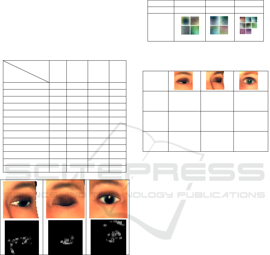
Table 7: First layer kernels learned for each network
described in Table 5.
Network Net1 Net2 Net3
Kernel 15x15 15x15 11x11
First
kernel
C1
Table 8: Networks responses (predictions) for simulated
image exemplars representing different eye states (C:
“closed”, O: “opened”, P: “partially opened”).
Table 7 shows the kernels learned in the C1 layer
of each network described in Table 5. It can be seen
that although the performance of the three
configurations are very similar, the learned kernels
are somewhat different. They all seem to perform a
similar tasks aiming at extracting simple point and
edge features. For example it can be seen that some
of the kernels resemble the typical characteristics of
the Laplacian of Gaussian (LoG) filter, when others
resemble oriented edge detection filters.
Table 8 shows the networks responses to sample
images, with the Net1 providing the highest decisions
confidence.
7 EYE BLINK DETECTION
As it has been mentioned, the eye status classification
and motion detection of the eyelids had been
frequently utilized before for a blink detection. Often,
these methods use a prior knowledge derived from the
test sets (in a simple case this could be a threshold
value) to be able to run the estimator (Fogelton,
Benesova, 2016). This may limit the applications of
such methods in a real environment. In the case of the
proposed approach the training data set is not linked
in any way with the data used for tests. Indeed
different databases were used for training (Helen) and
for testing (ZJU and Talking Face). This can make the
Net1
P:99.62%
O: 0.22%
C: 0.16%
P: 0.04%
O: 0.00%
C: 99.96%
P: 0.00%
O:100.0%
C: 0.00%
Net2
P: 90.60%
O: 0.01%
C: 9.40%
P: 7.32%
O: 0.30%
C: 92.38%
P: 0.00%
O:100.0%
C: 0.00%
Net3
P:71.73%
O: 27.48%
C: 0.79%
P: 24.44%
O: 0.19%
C:75.37%
P: 0.00%
O:100.0%
C: 0.00%
Online Eye Status Detection in the Wild with Convolutional Neural Networks
93

proposed approach more appropriate to work with the
data in the wild as in the case of the blink detection
test below.
Here, publicly available ZJU and Talking Face
(“Talking Face Video”) datasets, have been used for
the evaluation of the blink detection using the
proposed CNN model. A number of eye status
temporal sequences have been defined to represent
the blink action. For example, these include
sequences: “opened” - “closed” - “opened” or
“opened” - “partially opened” - “closed” - “opened”.
Table 9 lists the obtained results.
Table 9: Results obtained for blink detection using the
proposed method. PR: Precision, RE: Recall, GT: Ground
Truth, TP: True Positive, FP: False Positive. FN: False
Negative.
Dataset PR% RE% GT TP FP FN
ZJU 98 89.8 213 190 3 23
TF 100 100 55 55 0 0
Another advantage of using CNN in this case is
that the model is not sensitive to the subject motion.
Even if the eye images are blurred, due to the motion
of the subject as in Talking Face dataset, the model is
able to identify the eye status and subsequently the
blink action.
8 ONLINE IMPLEMENTATION
For an online implementation, the throughput of the
model should be fast enough to process the incoming
frames from the camera. The system that has been
used for online testing consists of PC with 1.2GHz 3i
CPU and 8GB memory, Nvidia GTX 960, and a
webcam. The method may also work without GPU
using CPU only. The processing starts with detecting
the face and then eye regions within 640x480 image.
This detection takes around 16ms, Table 10. When
GPU is used it takes on average 9.61ms to recognise
eye status, and 46.15ms if the algorithm is
implemented on CPU. This means that a video stream
with 15 fps can be processed in real-time on the CPU.
Table 10: Time required to detect the eye region using
Viola-Jones using CPU and recognise the eye status on
GPU and CPU.
Operation Time (ms)
Viola-Jones (CPU) 16.00
CNN model (GPU) 9.61
CNN model (CPU) 46.15
Figure 3 shows examples of the eye status
detection using the setup described above. It can be
seen that the system can predict the eye status with a
varied distance between the subject and the camera
and different head poses. This is because the model
has been trained on images with varied eye
representation, including pose and illumination.
Figure 3: CNN status detection snapshots.
9 CONCLUSIONS
This paper reports on a novel technique for the eye
status detection adopting convolutional neural
network (CNN) framework. It has been shown that
the proposed technique outperforms, on this problem,
the SVM method with SURF descriptors Bag of
Features and the AdaBoost with HOG and LBP
features. The eye dataset used in the testes is derived
from the Helen database which contains faces “in the
wild” including challenging cases with significant
illumination and head pose variability. Different
CNN configurations were tested and optimised to
show the dependence of the results on changes of
selected parameters of the network. The proposed eye
status detection method was further tested on the eye
blink detection problem. It has been shown that the
obtained results are comparable with the recently
reported state-of-the-art results. It should be
emphasised that the proposed method was trained on
the data derived from the Helen database. The
datasets used for blink detection evaluation, namely
ZJU and “Taking Face” were not used in any form for
the training of the method. This gives some
confidence that the proposed method would perform
in a similar way on other comparable data. Last but
not the least, it has been shown that the whole
processing pipeline, including eye detection and eye
status classification, can be performed in real-time.
ACKNOWLEDGMENT
Contributions to this paper by Bogdan Matuszewski
and Pedro Henriquez were supported by the European
Union Seventh Framework Programme (FP7/2013-
VISAPP 2017 - International Conference on Computer Vision Theory and Applications
94

2016) under grant agreement number 611516
(SEMEOTICONS).
REFERENCES
Fazli, S., Esfehani, P., 2012. Automatic Fatigue Detection
Based On Eye States. In: Proc. of Int. Conf. on
Advances in Computer Engineering.
Danisman, T., Bilasco, I., Djeraba, C., Ihaddadene, N.,
2010. Drowsy driver detection system using eye blink
patterns. In: Machine and Web Intelligence (ICMWI),
2010 International Conference on, pp. 230–233.
Divjak, M., Bischof, H., 2009. Eye blink based fatigue
detection for prevention of computer vision syndrome.
In: IAPR Conference on Machine Vision Applications,
pp. 350–353.
Drutarovsky, T., Fogelton, A., 2014. Eye blink detection
using variance of motion vectors. In: Computer Vision
- ECCV 2014 Workshops, Zurich, Switzerland.
Springer, Cham, Switzerland, pp. 436–448.
Du, Y., Ma, P., Su, X., Zhang, Y., 2008. Driver Fatigue
Detection based on Eye State Analysis. In: Proceedings
of the 11
th
Joint Conference on Information Sciences.
Fogelton, A., Benesova W., 2016. Eye blink detection
based on motion vectors analysis. Computer Vision and
Image Understanding, 148, 23-33.
Joshi, KV., Kangda, A., Patel, S., 2016. Real Time System
for Student Fatigue Detection during Online Learning”,
Inter. Jour of Hybrid Info. Tech.
Królak, A., Strumiłło, P., 2012. Eye-blink detection system
for human computer interaction. Universal Access Inf.
Soc. 11 (4), 409–419.
Le, V., Brandt, J., Lin, Z., Bourdev, L., Huang, T., 2012.
Interactive facial feature localization. ECCV’12,
pp.679-692.
LeCun, Y., Bottou, L., Bengio, Y., Haffner, P, 1998.
Gradient-based learning applied to document
recognition. Proceedings of the IEEE, pp. 2278—2324.
Lee, WO., Lee, EC., Park, KR., 2010. Blink detection
robust to various facial poses. In: J. Neurosci. Methods
193 (2), 356–372.
Liu, X., Tan, X., Chen, S., 2012. Eyes closeness detection
using appearance based methods. Springer,
International Conference on Intelligent Information
Processing, 398-408.
Malik, K., Smolka, B., 2014. Eye blink detection using
local binary patterns. In: 2014 International Conference
on Multimedia Computing and Systems (ICMCS), pp.
385–390.
Marcos-Ramiro, A., Pizarro-Perez, D., Marron-Romera,
M., Gatica-Perez., D., 2014. Automatic Blinking
Detection Towards Stress Discovery. In: Proc. of the
16th Int. Conf. on Multimodal Interaction, pp. 307—310.
Mohammed, A., Anwer, S., 2014. Efficient Eye Blink
Detection Method for disabled-helping domain. Inter.
Jour. of Adv. In: Computer Science and Applications.
Pan, G., Sun, L., Wu, Z., Lao, S., 2007. Eyeblink-based
anti-spoofing in face recognition from a generic
webcamera. In: 11
th
IEEE International Conference on
Computer Vision. ICCV ‘07, pp. 1–8.
Rezaei, M., Klette, R., 2012. Novel Adaptive Eye Detection
and Tracking for Challenging Lighting Conditions.
Asian Conference on Computer Vision, 427-440.
Portello, JK., Resenfield, M., Chu, CA., 2013. Blink Rate,
Incomplete Blinks and Computer Vision Syndrome.
Optometry and Vision Science, 90 (5), 4 82–4 87.
Saragih, JM., Lucey, S., Cohn, JF., 2011. Deformable
model fitting by regularized landmark mean-shift,
International Journal of Image and Vision
Computing, Vol. 91, Issue 2, pp 200–215.
Shin, HC., Roth, HR, Gao, M., Lu, L. Xu, Z., Nogues, I.,
Yao, J., Mollura, D., Summers, R., 2016. Deep
Convolutional Neural Networks for Computer-Aided
Detection: CNN Architectures, Dataset Characteristics
and Transfer Learning.
Sun, Y., Zafeiriou, S., Pantic, M., 2013. A Hybrid System
for On-line Blink Detection. In: Hawaii International
Conference on System Sciences.
Szwoch, M., Pieniazek, P., 2012. Eye blink based detection
of liveness in biometric authentication systems using
conditional random fields. In: Computer Vision and
Graphics. In: Lecture Notes in Computer Science,
7594. Springer, pp. 669–676.
“Talking Face Video”, Face & Gesture Recognition
Working Group, IST-2000-26434 http://www-prima.
inrialpes.fr/FGnet/data/01-TalkingFace/talking_face.
html.
Tomasi, C., Kanade, T., 1991. Detection and Tracking of
points features. Computer Science Department,
Carnege Mellon University, Tech. rep.
Viola, P., Jones, M., Polatsek, P., 2004. Robust real-time
face detection. International. Journal of Computer
vision. 57 (2), 137-154.
Wascher, E., Heppner, H., Möckel, T., Kobald, SO.,
Getzmann, S., 2015. Eye-blinks in choice response
tasks uncover hidden aspects of information processing.
In: Jour. Citation Reports, pp. 1207-1218.
Yosinski, J., Clune, J., Nguyen, A., Fucks, T., Lipson, H.,
2015. Understanding Neural Networks Through Deep
Visualization. In: Deep Learning Workshop, 31
st
International Conference on Machine Learning.
Online Eye Status Detection in the Wild with Convolutional Neural Networks
95