
Moving Object Detection by Connected Component Labeling of
Point Cloud Registration Outliers on the GPU
Michael Korn, Daniel Sanders and Josef Pauli
Intelligent Systems Group, University of Duisburg-Essen, 47057 Duisburg, Germany
{michael.korn, josef.pauli}@uni-due.de, daniel.sanders@stud.uni-due.de
Keywords:
3D Object Detection, Iterative Closest Point (ICP), Point Cloud Registration, Connected Component Labeling
(CCL), Depth Images, GPU, CUDA.
Abstract:
Using a depth camera, the KinectFusion with Moving Objects Tracking (KinFu MOT) algorithm permits
tracking the camera poses and building a dense 3D reconstruction of the environment which can also contain
moving objects. The GPU processing pipeline allows this simultaneously and in real-time. During the recon-
struction, yet untraced moving objects are detected and new models are initialized. The original approach to
detect unknown moving objects is not very precise and may include wrong vertices. This paper describes an
improvement of the detection based on connected component labeling (CCL) on the GPU. To achieve this,
three CCL algorithms are compared. Afterwards, the migration into KinFu MOT is described. It incorpo-
rates the 3D structure of the scene and three plausibility criteria refine the detection. In addition, potential
benefits on the CCL runtime of CUDA Dynamic Parallelism and of skipping termination condition checks are
investigated. Finally, the enhancement of the detection performance and the reduction of response time and
computational effort is shown.
1 INTRODUCTION
One key skill to understand complex and dynamic en-
vironments is the ability to separate the different ob-
jects in the scene. During a 3D reconstruction the
movement of the camera and the movement of one or
several observed objects not only aggravate the reg-
istration of the data over several frames, but on the
other hand further information for the decomposition
of the elements of the scene can be obtained, too. This
paper focuses on the detection of moving objects in
depth images on the GPU in real-time. In context
of this paper two phases of the reconstruction pro-
cess are distinguished: Firstly, the major process of
tracking and construction of models of all known ob-
jects and the static background (due to camera mo-
tion) of the scene. Typically, depth images are pro-
cessed as point clouds and tracking can be accom-
plished by point cloud registration by the Iterative
Closest Point (ICP) algorithm, which is a well-studied
algorithm for 3D shape alignment (Rusinkiewicz and
Levoy, 2001). Afterwards, the models can be cre-
ated and continually enhanced by fusing all depth im-
age data into voxel grids (Curless and Levoy, 1996).
Secondly and focused in this paper, after the registra-
tion of each frame the data must be filtered for new
moving objects for which no models have been pre-
viously considered. Obviously, all pixels which can
be matched sufficiently with existing models do not
indicate a new object. But pixels that remained as
outliers of the registration process may be caused by
a yet untraced moving object. Likewise, outliers are
spread over the whole depth data due to sensor noise,
reflection, point cloud misalignment, et cetera. Ac-
cordingly, just large clusters (in the three-dimensional
space) of outliers can be candidates for the initializa-
tion of a new object model. These clusters can be
found by Connected Component Labeling (CCL) on
the GPU. Subsequently, the shape of the candidates
has to be verified with some plausibility criteria.
This paper is organized as follows. In section 2
the required background knowledge concerning the
3D reconstruction process is summarized. In addi-
tion, in subsection 2.3 the detection of new objects is
discussed especially. At the beginning of section 3,
three GPU based CCL algorithms are introduced and
compared. Afterwards the migration into an existing
3D reconstruction algorithm is described and two fur-
ther runtime optimizations are discussed. Section 4
details our experiments and results. In the final sec-
tion we discuss our conclusions and future directions.
Korn M., Sanders D. and Pauli J.
Moving Object Detection by Connected Component Labeling of Point Cloud Registration Outliers on the GPU.
DOI: 10.5220/0006173704990508
In Proceedings of the 12th International Joint Conference on Computer Vision, Imaging and Computer Graphics Theory and Applications (VISIGRAPP 2017), pages 499-508
ISBN: 978-989-758-227-1
Copyright
c
2017 by SCITEPRESS – Science and Technology Publications, Lda. All rights reserved
499

2 BACKGROUND
Our implementation builds on the KinectFusion
(KinFu) algorithm which was published in (Izadi
et al., 2011; Newcombe et al., 2011) and has become
a state-of-the-art method for 3D reconstruction in the
terms of robustness, real-time and map density. The
next subsection outlines the original KinFu publica-
tion. Afterwards, an enhanced version is introduced.
Finally, the detection of new moving objects is de-
scribed in detail.
2.1 KinectFusion
The KinectFusion algorithm generates a 3D recon-
struction of the environment on a GPU in real-time
by integrating all available depth images from a depth
sensor into a discretized Truncated Signed Distance
Functions (TSDF) representation (Curless and Levoy,
1996). The measurements are collected in a voxel grid
in which each voxel stores a truncated distance to the
closest surface including a related weight that is pro-
portional to the certainty of the stored value. To inte-
grate the depth data into the voxel grid every incom-
ing depth image is transformed into a vertex map and
normal map pyramid. Another deduced vertex map
and normal map pyramid is obtained by ray casting
the voxel grid based on the last known camera pose.
According to the camera view, the grid is sampled by
rays searching in steps for zero crossings of the TSDF
values. Both pyramids are registered by a ICP proce-
dure and the resulting transformation determines the
current camera pose. Due to runtime optimization the
matching step of the ICP is accomplished by projec-
tive data association and the alignment is rated by a
point-to-plane error metric (see (Chen and Medioni,
1991)). Subsequently, the voxel grid data is updated
by iterating over all voxels and the projection of each
voxel into the image plane of the camera. The new
TSDF values are calculated using a weighted running
average. The weights are also truncated – allowing
the reconstruction of scenes with some degree of dy-
namic objects. Finally, the maps, created by the ray-
caster, are used to generate a rendered image of the
implicit environment model.
2.2 KinectFusion with Moving Objects
Tracking
Based on the open-source publication of KinFu, re-
leased in the Point-Cloud-Library (PCL; (Rusu and
Cousins, 2011)), Korn and Pauli extended in (Korn
and Pauli, 2015) the scope of KinFu to the ability to
reconstruct the static background and several moving
rigid objects simultaneously and in real-time. Inde-
pendent models are constructed for the background
and each object. Each model is stored in its own voxel
grid. During the registration process for each pixel
of the depth image the best matching model among
all models is determined. This yields a second out-
put of the ICP beside the alignment of all existing
models: the correspondence map. This map contains
the assignment of each pixel of the depth image to a
model or information why the matching failed. First
of all, the correspondence map is needed to construct
the equation systems which minimize the alignment
errors. Afterwards, it is used to detect new moving
objects. It is highly unlikely that during the initial de-
tection of an object the entire shape and extent of the
object can be observed. During the processing of fur-
ther frames the initial model will be updated and ex-
tended. Because of this the initial allocated voxel grid
may turn out as too small and therefore, the voxel grid
will grow dynamically in this case.
2.3 Detection of New Moving Objects
The original detection approach from (Korn and
Pauli, 2015) is illustrated in Fig. 1 by the com-
puted correspondence maps. The figure shows cho-
sen frames from a dataset recorded with a handheld
Microsoft Kinect for Xbox 360. In the center of the
scene, a middle size robot with a differential drive and
caster is moving. On an aluminum frame a laptop, a
battery and an open box on the top is transported. At
first most pixels can be matched with the static back-
ground model. Then more and more registration out-
liers occur (dark and light red). In addition, potential
outliers (yellow) were introduced in (Korn and Pauli,
2015). These are vertices with a point-to-plane dis-
tance that is small enough (< 3.5 cm) to be treated as
inlier in the alignment process. On the other hand, the
distance is noticeable large (> 2 cm) and such match-
ings cannot be considered as totally certain. Because
of this, potential outliers are processed like outliers
during the detection phase.
The basic idea of the detection is that small accu-
mulations of outliers can occur due to manifold rea-
sons. But large clusters are mainly caused by move-
ment in the scene. The detection in (Korn and Pauli,
2015) is performed window-based for each pixel. The
neighborhood with a size of 51 × 51 pixels of each
marked outlier is investigated. If 90% of the neigh-
bor pixels are marked as outliers or potential outliers,
then the pixel in the center of the window is marked as
new moving object. In the next step, each (potential)
outlier in a much smaller 19 × 19 neighborhood of a
pixel marked as a moving object is also marked as a
VISAPP 2017 - International Conference on Computer Vision Theory and Applications
500

Figure 1: The first image provides an overview of a substantial part of the evaluation scene. The remaining images show the
Visualization of the correspondence maps of the frames 160 to 173 (row-wise from left to right) of a dataset which contains
a moving robot in the center of the scene. Each correspondence map shows the matched points with the background (light
green), the matched points with the object (dark green), potential outlier (yellow), ICP outlier (dark red), potential new object
(light red), missing points in depth image (black) and missing correspondences due to volume boundary (blue).
moving object. Subsequently, the found cluster is ini-
tialized as new object model (dark green in frame 168
in Fig. 1)), including the allocation of another voxel
grid, if three conditions are met. Particularly, a mov-
ing object needs to be detected in at least 5 of the con-
secutive previous frames (frames 163-167 in Fig. 1).
Two further requirements concern environments with
several moving objects. However, these are behind
the scope of this paper due to the focus on the de-
tection phase. This detection strategy has three core
objectives:
• The initial model size must be extensive enough to
provide sufficient 3D structure for the following
registration process. In the original approach of
Korn and Pauli the minimal size is approximately
19 × 19 pixels.
• The initial model may not include extraneous
vertices. This is the major weakness of the imple-
mentation in (Korn and Pauli, 2015) since the de-
tection does not depend on the 3D structure (e.g.
the original vertex map). Vertices from surfaces
far away from the moving object may get part of
the cluster of outliers even though they are not
connected in 3D. This happens likely at the bor-
ders of the object, wherefore a margin of not used
outliers exists (light red is enclosed by dark red in
Fig. 1). It should be noted that the algorithm is
almost always working even if a few wrong out-
liers are assigned to the object, but the initial voxel
grid is much too large and the performance (video
memory and runtime) decreases.
• The appearance of a new object should be sta-
ble. A detection based on just one frame would
be risky. If large clusters of outliers are found in
5 sequential frames, a detection is much more re-
liable. The time delay of 5 · 33 ms = 165 ms is
bearable, but the reconstruction process also mis-
assigns the information of 5 frames. This is par-
tially compensated because the detected clusters
are likely to be larger in subsequent frames and
they should at least contain the vertices of the pre-
vious frames (compare frame 163 with 167). The
lost frames could also be buffered and reprocessed
but this would not be real-time capable with cur-
rent GPUs.
In the remaining parts of this paper the improve-
ment of the detection process is investigated. By de-
ciding on each particular vertex, whether it belongs
to the largest cluster of outliers or not, the first two
points of the list above can be enhanced. By incor-
porating the 3D structure, the inclusion of extrane-
ous vertices is prevented and the full size of the clus-
ters can be determined. Seed-based approches (e.g.
region growing) are unfavorable on a GPU. Further-
more, it would be necessary to find good seed points
which would increase the computational effort. How-
ever, several CCL algorithms were presented which
are optimized for the GPU architecture and able to
preserve the real-time capability of KinFu.
Moving Object Detection by Connected Component Labeling of Point Cloud Registration Outliers on the GPU
501

3 CONNECTED COMPONENT
LABELING ALGORITHMS
In order to develop a CCL algorithm, that works on
correspondence maps and incorporates the 3D struc-
ture, three CCL on GPU algorithms are briefly intro-
duced in the next subsections. More details and pseu-
docode can be found in the referenced papers. Sub-
sequently, the algorithms are compared and our algo-
rithm is derived. For the beginning, a binary input for
the CCL algorithms is assumed. A correspondence
map can be reduced to a binary image: A pixel is
a (potential) outlier or not. A label image (or label
array) is the result of all CCL algorithms, in which
each pixel is labeled with the component ID. All pix-
els with the same ID are direct neighbors or they are
recursively connected in the input data. In the last
subsection, depth information are additionally inte-
grated.
3.1 Label Equivalence
Hawick et. al. give in (Hawick et al., 2010) an
overview of several parallel graph component label-
ing algorithms with GPGPUs. This subsection sum-
marizes the label equivalence method (Kernel D in
(Hawick et al., 2010)) which uses one independent
thread on the GPU for the processing of each pixel.
One input array D
d
is needed, which assigns a class
ID to each pixel. In our case just 1 (outlier) or 0
(anything else) are used but more complex settings
are possible, too. Before the start of an iterative pro-
cess, a label array L
d
is initialized. It stores the label
IDs for each pixel and all pixels start with their own
one-dimensional array index (see left side of Fig. 2).
Furthermore, a reference list R
d
is allocated which is
a copy of L
d
at the beginning. The iterations of this
method are subdivided in three GPU kernels:
• Scanning: For each element of L
d
the smallest
label ID in the Von Neumann neighborhood (4-
connected pixels) with similar class ID in D
d
is
searched (see red arrows in Fig. 2). If the found
ID is smaller than the original ID, which was
stored for the processed element in L
d
, the result
is written into the reference list R
d
at the position
which is referenced by the current element in L
d
.
This means the root node of the current connected
component is updated and hooked into the other
component and not just the current node. Since
several threads may update the root node concur-
rently atomicMin is used by Hawick et. al. We
waive this atomic operation because it increases
the runtime. Without this operation sometimes the
update of a root node is not optimal and an addi-
0
1 2
3
4
5 6
7
8
9
10
11 12
13
14
15 16
17
18
19
20
21 22
23
24
0 0 0 3 3
5 0 0 0 3
5 5 0 13 3
15 15 0 13 3
15 15
22
13 3
Figure 2: Visualization of a single iteration of the label
equivalence algorithm. The background color (light gray
or dark gray) represents the class of each pixel. Red arrows
show the results of the scanning phase. Blue arrows show
the results of the analysis phase. The left part of the figure
illustrates the initial labels in L
d
and the right part the la-
bels after running the labeling kernel at the end of the first
iteration. The red arrows on the right side additionally in-
dicate how the root nodes of the connected components are
updated during the scanning phase of the second iteration.
tional iteration is maybe necessary, but in general
this costs less than the repeated use of an expen-
sive atomic operation.
• Analysis: The references of each element of the
reference list R
d
are resolved recursively until the
root node is reached (see blue arrows in Fig. 2).
For example position 7 gets the assignment 0 in
Fig. 2 due to the reference chain 7 → 2 → 1 →
0. Element 0 is a root node because it references
itself.
• Labeling: The labeling kernel updates the label-
ing in L
d
by copying the results from the reference
list R
d
(right side of Fig. 2).
The iterations terminate if no further modification ap-
pears during the scanning phase.
3.2 Improved Label Equivalence
Based on the label equivalence method, Kalentev
et. al propose in (Kalentev et al., 2011) a few im-
provements in terms of runtime and memory require-
ments. The reference list R
d
is replaced by writing the
progress of the scanning and analysis phases directly
into the label array L
d
. This also makes the whole
labeling step obsolete. Besides the obvious memory
saving, it can reduce the computational effort, too.
Some threads may benefit from updates in L
d
made
by other threads. Additionally, the original input data
is padded with a one pixel wide border. This allows
to remove the if conditioning in the scanning phase
which checks the original image borders. Further-
more, it makes the ID 0 free to mark irrelevant back-
ground pixels, including the padded area. Kalentev
et. al also removed D
d
, due to this only two classes of
pixels are considered: unprocessed background pixels
VISAPP 2017 - International Conference on Computer Vision Theory and Applications
502

Merging scheme
LEVEL = 0
LEVEL = LEVEL + 1
Labeled
output data
LEVEL = =
Top level?
Kernel 4
Update all labels
Kernel 2
Merge solution
on borders (LEVEL)
Kernel 1
Solve CCL subproblem
in shared memory
Input data
Kernel 3
Update labes on
borders (LEVEL)
0
1
Figure 3: Schematic overview of the hierarchical merging
approach (
ˇ
S
´
tava and Bene
ˇ
s, 2010).
and connected foreground pixels. Finally, Kalentev
et. al proposed to avoid the atomicMin as described
in the previous subsection, too.
3.3 Hierarchical Merging CCL
ˇ
S
´
tava and Bene
ˇ
s published in (
ˇ
S
´
tava and Bene
ˇ
s, 2010)
a CCL algorithm which is specifically adapted to the
GPU architecture. In particular, Kernel 1 (see Fig. 3)
applies the improved label equivalence method within
the shared memory of the GPU. This memory type
can just be used block wise and the size is very lim-
ited and therefore Kernel 1 processes the input data
in small tiles. Then Kernel 2 merges the components
along the border of the tiles by updating the root node
with the lower ID. Subsequently, the non-root nodes
along the borders are updated by the optional Kernel 3
which enhances the performance. All tiles are merged
hierarchically with much concurrency. Finally, Ker-
nel 4 flats each equivalence tree with an approach
similar to the analysis phase of the label equivalence
method. The main disadvantage lies in the limited for-
mats of the input data. The implementation of
ˇ
S
´
tava
and Bene
ˇ
s only works with arrays that have a size of
power of two in both dimensions. In addition, just
quadratic images run with the reference implemen-
tation provided with the online resources of (
ˇ
S
´
tava
and Bene
ˇ
s, 2010). The original publication detects
connected components with the Moore neighborhood
but we reduced it to the neighborhood with just 4-
connected pixels. This improves the performance and
the impact on the quality of the the results is negligi-
ble.
3.4 Comparison between the CCL
Algorithms
All three CCL algorithms provide substantially deter-
ministic (just the IDs of the components can change)
and correct results. The runtimes of the algorithms
were compared with three categories of test images
without depth information shown in Fig. 4. The first
image was generated by binarization of a typical cor-
respondence map with a moving robot slightly left of
the image center. In addition, two more extensive cat-
egories of test images were evaluated to find an upper
correspondence map
random circles
spiral
Figure 4: Test images for the comparision of the runtime of
the three CCL algorithms.
limit of the runtime effort. Since KinFu runs in real-
time, not only the average runtime with typical outlier
distributions is interesting, but also the worst case lag
(response time), because this could let the ICP fail.
Images with random circles represent situations with
many outlier pixels which are very unlikely but pos-
sible, for example after fast camera movements. The
spiral is deemed to be a worse case scenario for CCL
algorithms. The connectivity of the spiral must be
traced with very high effort over the entire image and
in all directions (left, right, top and down).
The runtimes are measured with an Intel Core i7-
2600 @3.40GHz, DDR3 SDRAM @1600MHz and
a Nvidia GeForce GTX970. The time for memory
allocation and transfers of the input and output data
between the host and the device was not measured.
These operations depend in general on the applica-
tion and in KinFu MOT the input and output data just
exist in the device memory. The evaluation was per-
formed for several resolutions so that it is usable for
higher depth camera resolutions in the future or other
applications. Due to the limitations of the hierarchi-
cal merging CCL algorithm only square images were
used. The correspondence map test image was scaled
with nearest neighbor interpolation.
Fig. 5(a) shows the runtimes with the binary corre-
spondence map. The algorithm of Hawick et. al. per-
forms worst and the hierarchical merging CCL overall
best. It is noticeable that the runtime of the hierar-
chical merging CCL can decrease with increasing im-
age size (compare 1664
2
with 1792
2
pixels). Fig. 5(b)
highlights that all algorithms suffer from highly occu-
pied input images. Particularly, the hierarchical merg-
ing CCL loses its lead and it is partially outperformed
Moving Object Detection by Connected Component Labeling of Point Cloud Registration Outliers on the GPU
503

256
2
512
2
768
2
1024
2
1280
2
1536
2
1792
2
2048
2
0.1
1
10
size of input image [pixel]
avg. runtime [ms]
(a) correspondence map
256
2
512
2
768
2
1024
2
1280
2
1536
2
1792
2
2048
2
0.1
1
10
size of input image [pixel]
avg. runtime [ms]
(b) random circles
256
2
512
2
768
2
1024
2
1280
2
1536
2
1792
2
2048
2
0.1
1
10
size of input image [pixel]
avg. runtime [ms]
(c) spiral
Label Equivalence
Improved Label Equivalence
Hierarchical Merging CCL
Figure 5: Runtimes of the CCL algorithms with different
images and resolutions. The runtimes are logarithmical
scaled and the averages of 100 runs are shown.
by improved label equivalence.
ˇ
S
´
tava and Bene
ˇ
s al-
ready noted in their paper that their algorithm per-
forms best when the distribution of connected compo-
nents in the analyzed data is sparse. In Fig. 5(c) im-
proved label equivalence shows the overall best result.
The algorithm of
ˇ
S
´
tava and Bene
ˇ
s has major trouble
to resolve the high number of merges.
As expected, the basic label equivalence algorithm
is outperformed by the other two. But the runtime dif-
ferences need to be put in context. Hawick et. al. use
an array D
d
to distinguish between classes or e.g. dis-
tances. It makes this algorithm more powerful than
the other two and it is very near to our aim to use
depth information during the labeling. The effort for
using D
d
should not be underestimated – the addi-
tional computations are low-cost, but the device mem-
ory bandwidth is limited.
To determine the best basis of our KinFu MOT
extension, we need to take a closer look at the possi-
ble input data sizes. The size of the correspondence
maps in the intended application is the same as the
size of the depth images. The depth image resolu-
tion of the Kinect for Xbox 360 is 640 × 480 pixels.
Because of the structured light technique, the men-
tioned resolution is far beyond the effective resolution
of the first Kinect generation. As a further example,
the Kinect for Xbox One has a depth image resolution
of 512 ×424 pixels which can be assumed as effective
due to the time-of-flight technique.
The input data formats of the reference implemen-
tation of
ˇ
S
´
tava and Bene
ˇ
s are very restricted and it
would be necessary to pad the correspondence maps
in KinFu MOT. Therefore, runtimes with sparse VGA
resolution inputs are slightly better with improved la-
bel equivalence than hierarchical merging CCL. Ad-
ditionally, the runtimes of the hierarchical approach
may rise more with dense input data and the complex
source code is hard to maintain or modify. Altogether
the improved label equivalence algorithm is a good
basis for the detection of moving objects in KinFu
MOT.
3.5 Migration into KinFu MOT
Our enhancement of KinFu MOT is primary based on
the improved label equivalence method from subsec-
tion 3.2. The input label array is initialized on the ba-
sis of the latest correspondence map. Pixels marked
as outlier or potential outlier get the respective array
index and all other get 0 (background) as label ID.
In addition, the scanning kernel relies on the current
depth image (bound into texture memory) during the
neighborhood search. Two neighbor pixels are only
connected if the difference of their depth values is
VISAPP 2017 - International Conference on Computer Vision Theory and Applications
504

smaller than 1 cm. This threshold seems very low
but to establish a connection, one path out of several
possible paths is sufficient. If one element of the Von
Neumann neighborhood does not pass the threshold
due to noise, then probably one of the remaining three
will pass. Furthermore, the padding with a one pixel
wide border is removed because the additional effort
is too much for small images. In our case it would be
necessary to pad the input label array and the depth
image and remove the padding again from the output
label array.
Just the largest component is considered for an ob-
ject initialization. To find it, a summation array of the
same size as the label array is initialized with zeros.
Each element of the output label array is processed
with its own thread by a summation kernel. For IDs
6= 0 the summation array at index = ID is incremented
with atomicAdd. The maximum is found with paral-
lel reduction techniques. In contrast to conventional
implementations a second array is needed to carry the
ID of the related maximum value.
The average runtime with VGA resolution inputs
with the described implementation (without the mod-
ifications which are presented below) is 43% higher
than the runtime of the improved label equivalence
method from subsection 3.2. This is caused by the
additional effort for incorporating depth information
and particularly for the determination of the largest
component.
3.5.1 Dynamic Parallelism
One bottleneck of the label equivalence approach is
the termination condition. To check if a further it-
eration should be performed, the host needs a syn-
chronous memory copy to determine if modifications
appear during the last scanning phase. With CUDA
compute capability 3.5, Dynamic Parallelism was in-
troduced which allows parent kernels to launch nested
child kernels. The obvious approach is to replace
the host control loop by a parent kernel with just
one thread. The synchronization between host and
device can be avoided, but unfortunately cudaDe-
viceSynchronize must be called in the parent kernel
to get the changes from the child kernels. Altogether,
this idea turned out to be slower than the current ap-
proach. Over all image sizes the runtime of the bare
CCL algorithm rises by approx. 10% (measured with-
out component size computation and outside of KinFu
MOT). Due to using streams in KinFu MOT cudaDe-
viceSynchronize can have an even worse impact. Dy-
namic Parallelism was removed from the final imple-
mentation.
3.5.2 Effort for Modification Checking
The effort for modification checking within the scan-
ning phase can be reduced if further CCL iteration are
executed without verification of the termination con-
dition. Fig. 2 shows that, even in the case of simple
input data, two interation are necessary. During our
evaluation on real depth images mostly three CCL
iterations are needed and always not less than two.
Accordingly, the second iteration can be launched di-
rectly after the first iteration without checking the
condition. This reduces the runtime by approx.
0.01 ms (4.2% with VGA resolution) with the corre-
spondence map. If the second condition check is also
dropped, the runtime is reduced by approx. 7.2%.
3.5.3 Plausibility Criteria
To prevent bad object initializations three criteria are
verified in addition to the preconditions, which were
mentioned in subsection 2.3.
At first, the size of the largest found component
must exceed a threshold. Only clusters of ouliers with
sufficient elements are supposed to be caused by a
moving object. Additionally, dropping false negatives
is not a drawback in this case, since the following
point cloud registration can fail without sufficient 3D
structure. Checking the first criterion is very conve-
nient because the size is previously calculated to find
the largest component. If it is fulfilled, then additional
effort has to be spent for the other two criteria.
It would be valuable to calculate the oriented
bounding box (OBB) for the component and demand
a minimum length of the minor axis and use a thresh-
old for the filling degree. But the computation of
a OBB takes too much runtime. This idea is re-
placed by two other characteristics which admittedly
are slightly worse rotational invariant but faster.
For each row i of the label array an additional
CUDA kernel determines the first
x
f irst
i
and the last
x
last
i
column index which belongs to the found com-
ponent. Moreover, rowsSet counts the number of
rows which contain at least one element of the compo-
nent and
x
f irst
i
=
x
last
i
= 0 for empty rows. A further
kernel does the same for all columns of the label array,
which yields to
y
f irst
j
,
y
last
j
and colsSet. The sec-
ond critertia is met if the relation between the number
of elements of the component componentPixels and
the approximated occupied area
2 · componentPixels
rows−1
∑
i=0
x
last
i
−
x
f irst
i
+
cols−1
∑
j=0
y
last
j
−
y
f irst
j
(1)
exceeds a threshold of 75%, where rows and cols
specify the dimensions of the whole label array. This
Moving Object Detection by Connected Component Labeling of Point Cloud Registration Outliers on the GPU
505

(a) rejected by second criterion
(b) rejected by third criterion
Figure 6: Examples for shapes which are rejected by the
second and third criterion. The green lines indicate
x
last
i
−
x
f irst
i
and
y
last
j
−
y
f irst
j
for some rows and columns.
ensures that the filling degree is not too low and using
horizontal and vertical scans improves the rotational
invariance. The third criterion is fulfilled if the av-
erage expansions of the component in horizontal and
vertical direction
rows−1
∑
i=0
x
last
i
−
x
f ir st
i
rowsSet
and
cols−1
∑
j=0
y
last
j
−
y
f ir st
j
colsSet
(2)
are at least 15 pixels. This is useful to avoid thin but
long shapes which appear very often at the border be-
tween objects. Fig. 6 illustrates how both criteria take
effect on two different shapes. Particularly, example
(b) can be observed often due to misalignment of ta-
bles (shown in Fig. 6(b)) and doorframes.
4 EVALUATION AND RESULTS
In this section, the CCL based object detection is eval-
uated with regard to the detection results and runtimes
compared to the original procedure described in sub-
section 2.3. The evaluation is mainly based on six
datasets of one scene, which was introduced in sub-
section 2.3. The datasets differ in camera movement
and the path the robot took (reflected by the dataset
names). Finally, a qualitative Evaluation gives an im-
pression of the enhanced potential of KinFu MOT.
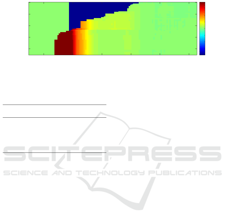
4.1 Detection Performance
The detection results are compared pixelwise based
on the correspondence maps in dependency of the
threshold for the minimal size of the found con-
nected component (first criterion in subsection 3.5).
The thresholds of the original approach remain un-
changed. Fig. 7 shows for several frames of dataset
robot frontal to camera the relative enhancement of
the new CCL based algorithm
enh =
(
nCCL+nCommon
nOrig+nCommon
− 1, if nCCL ≥ nOrig
−
nOrig+nCommon
nCCL+nCommon
+ 1, otherwise
,
(3)
where nCommon is the count of pixels which are
marked as found moving object by the new and the
original approach, nCCL counts pixels only assigned
by the new process and nOrig is the count detected
exclusively by the original approach. The scale of
enh is clipped at −4 and 4 and division by 0 in Equa-
tion 3 is meaningfully solved. After the object ini-
tialization, the object model is continually extended
by the reconstruction process and the counted pixels
depend only indirectly on the detection. The shown
heatmap is representative for all six datasets. The
original KinFu MOT algorithm initializes the robot
model with 11.2% of the ground truth object pixels
at frame 138. With a size threshold ≤ 5000 pixels
the proposed approach initializes the robot between
frame 124 (31.6% of the object pixels) and 136 (dark
red area). Even after frame 138, the object size de-
tected by the original approach needs a few frames to
reach the results of the new approach (gradient from
dark red via red, orange, yellow to green). For larger
size thresholds the detection is delayed (dark blue) but
the original algorithm is caught up immediately (in-
stantly from dark blue to green) or even outperformed
(dark blue to orange, yellow and green).
In our experiments the size threshold is the most
important parameter. If it is too small, tiny com-
ponents can be detected as moving objects without
containing sufficient 3D structure for the registration,
or they are even false positives. A high threshold
unnecessarily delays the detection. Altogether, the
new approach is never worse than the original algo-
rithm which is mostly outperformed. The heatmaps of
the other datasets support the described observations.
The specific characteristics of the stepped shape of the
heatmaps differ but the conclusions are similar. Over
all datasets, 3500 pixels is a suitable size threshold.
4.2 Runtime Performance
Table 1 shows that in comparison with the original
approach in KinFu MOT, the runtime is reduced by
VISAPP 2017 - International Conference on Computer Vision Theory and Applications
506
120 140 160 180 200 220
frame number
2000
4000
6000
8000
10000
minimal size threshold
-4
-3
-2
-1
0
1
2
3
4
relative enhancement
Figure 7: The relative enhancement of the new CCL based algorithm compared to the original approach in dependency of the
size threshold and frame number.
Table 1: Total runtimes with SD for the object detection
of the proposed process described in subsection 3.5 and the
original approach in KinFu MOT described in (Korn and
Pauli, 2015).
Dataset avg. runtime per frame[ms]
CCL based original approach
parallel to image plane 0.85 ± 0.22 1.69 ± 0.38
robot towards camera 0.71 ± 0.32 1.15 ± 0.21
robot frontal to camera 0.63 ± 0.17 1.72 ± 0.27
robot away from camera 0.56 ± 0.12 1.10 ± 0.23
complete robot pass 0.55 ± 0.10 1.10 ± 0.28
robot rotation 0.53 ± 0.09 1.24 ± 0.32
the new approach, despite the higher complexity of
the algorithm. This can be traced back to the exten-
sive access of the global memory of the original ap-
proach. Overall the standard deviation (SD) is slightly
reduced, too. While the SD of the original approach is
dominated by the amount of registration outliers, this
influence is less important for the proposed process.
Mostly the SD of the CCL based approach depends
on the number of large connected components which
pass the first criterion and trigger the computation of
the other two criteria. This observation is particularly
supported by the first dataset in Fig. 8. Overall, in the
datasets with more detection effort, it is very difficult
to register the moving robot with the model because
mainly parallel planes are first visible (especially in
the upper three datasets) and the alignment is instable
due to the point-to-plane metric of KinFu. Large out-
lier regions occur frequently and criteria 2 and 3 have
to be computed. In summary, Table 1 shows that the
response time is roughly halved. But this reflects the
computational effort insufficiently due to many syn-
chronizations between the host and device in the pro-
posed approach. The underlying data of Fig. 8 indi-
cates that the total GPU computation time for all ker-
nels is approximately quartered in comparison with
the original approach in KinFu MOT described in
(Korn and Pauli, 2015). The GPU time for the first
600 frames was reduced from 869 ms to 272 ms for
parallel to image plane and from 980 ms to 174 ms
for robot frontal to camera.
4.3 Qualitative Evaluation
The newer Kinect for Xbox One provides very chal-
lenging data. The dataset in Fig. 9 was created with
a system for optical inspection, which can be seen as
a three-dimensional cartesian robot. First, it was re-
quired to extend KinFu with a model for radial cam-
era distortion. In addition, the higher spatial depth im-
age resolution yields much details but the data contain
excessive noise and reflections. Due to the complex
shapes of the outlier clusters, the original detection
approach mostly fails. The new CCL approach suc-
cessfully leads to one background model and three
additional object models (the three moved axes of
the robot). The impact of sensory distortions is re-
duced because the component connectivity is deter-
mined based on the depth data, too. Besides, the de-
tection does not demand on square regions of outliers
with 90% filling degree which allow early object ini-
tializations.
5 CONCLUSIONS
It was ascertained that improved label equivalence,
proposed by Kalentev et. al, behaves well on the
GPU with small images like common depth images.
Whereas the hierarchical merging CCL algorithm
does not bring any benefits for small images and its
performance even declines if the data is not sparse.
A Dynamic Parallelism approach leads to a increased
runtime of label equivalence algorithms. However,
the response time can be reduced by skipping the first
two verifications of the termination condition.
The migration in KinFu MOT was extended by a
search for the largest component and three criteria.
Moving Object Detection by Connected Component Labeling of Point Cloud Registration Outliers on the GPU
507

0
50
100
150
200
250
parallel to image plane
robot towards camera
robot frontal to camera
robot away from camera
complete robot pass
robot rotation
total runtime [ms]
Init
Scanning
Analysis
Criterion 1
Criteria 2&3
Figure 8: Comparison of the runtimes for six different datasets. Shown is the total runtime over the first 600 frames for
selected CUDA kernels (just GPU time). The first three kernels are mentioned in subsection 3.1. Criterion 1 shows the effort
for counting the size of each component and finding the maximum. Criteria 2 & 3 involves all kernels which are needed to
compute both criteria.
rgb overview correspondence map
rendered first object rendered background model
Figure 9: Reconstruction of three moving elements and the
background with the Kinect for Xbox One and the CCL
based detection. The four different green tones in the corre-
spondence map show four independent object models.
The decrement of the response time and computa-
tional effort was shown and the improvement of the
detection performance is conclusively. Additionally,
the depth data are considered and false connections
are inhibited which is a necessary extension for a re-
liable detection, especially in complex datasets.
For future work, the plausibility criteria should be
refined. Furthermore, the strategy for the stability ob-
jective mentioned in subsection 2.3 can be extended.
The large clusters of outliers which need to be found
in 5 sequential frames should match in position and
perhaps even shape. This is expensive because the
camera can be moved and the problem needs to be
solved in 3D.
REFERENCES
Chen, Y. and Medioni, G. (1991). Object modeling by reg-
istration of multiple range images. In Robotics and
Automation, 1991. Proceedings., 1991 IEEE Interna-
tional Conference on, pages 2724–2729 vol.3.
Curless, B. and Levoy, M. (1996). A volumetric method for
building complex models from range images. In Pro-
ceedings of the 23rd Annual Conference on Computer
Graphics and Interactive Techniques, SIGGRAPH
’96, pages 303–312, New York, NY, USA. ACM.
Hawick, K. A., Leist, A., and Playne, D. P. (2010). Parallel
Graph Component Labelling with GPUs and CUDA.
Parallel Computing, 36(12):655–678.
Izadi, S., Kim, D., Hilliges, O., Molyneaux, D., Newcombe,
R., Kohli, P., Shotton, J., Hodges, S., Freeman, D.,
Davison, A., et al. (2011). KinectFusion: real-time 3D
reconstruction and interaction using a moving depth
camera. In Proceedings of the 24th annual ACM sym-
posium on User interface software and technology,
pages 559–568. ACM.
Kalentev, O., Rai, A., Kemnitz, S., and Schneider, R.
(2011). Connected component labeling on a 2D grid
using CUDA. Journal of Parallel and Distributed
Computing, 71(4):615–620.
Korn, M. and Pauli, J. (2015). KinFu MOT: KinectFu-
sion with Moving Objects Tracking. Proceedings of
the 10th International Conference on Computer Vision
Theory and Applications (VISAPP 2015).
Newcombe, R., Izadi, S., Hilliges, O., Molyneaux, D., Kim,
D., Davison, A. J., Kohi, P., Shotton, J., Hodges, S.,
and Fitzgibbon, A. (2011). KinectFusion: Real-time
dense surface mapping and tracking. In Mixed and
augmented reality (ISMAR), 2011 10th IEEE interna-
tional symposium on, pages 127–136. IEEE.
Rusinkiewicz, S. and Levoy, M. (2001). Efficient Variants
of the ICP Algorithm. In Proc. of the 3rd Interna-
tional Conference on 3-D Digital Imaging and Mod-
eling, pages 145–152.
Rusu, R. B. and Cousins, S. (2011). 3D is here: Point
Cloud Library (PCL). In International Conference on
Robotics and Automation, Shanghai, China.
ˇ
S
´
tava, O. and Bene
ˇ
s, B. (2010). Connected Component La-
beling in CUDA. Hwu., WW (Ed.), GPU Computing
Gems.
VISAPP 2017 - International Conference on Computer Vision Theory and Applications
508
