New Flow-based Heuristic for Search Algorithms Solving Multi-agent
Path Finding
Jiri Svancara
1
and Pavel Surynek
1,2
1
Faculty of Mathematics and Physics, Charles University, Prague, Czech Republic
2
National Institute of Advanced Industrial Science and Technology (AIST), Tokyo, Japan
Keywords:
Multi-agent Path Finding, A*, Heuristic Function, Multi-commodity Flow, Network Flow, Maximum Flow,
Makespan Optimality.
Abstract:
We address the problem of optimal multi-agent path finding (MAPF) in this paper. The task is to find a set
of actions for each agent in know terrain so that each agent arrives to its desired destination from a given
starting position. Agents are not allowed to collide with each other along their paths. Furthermore, a solution
that minimizes the total time is required. In this paper we study search-based algorithms that systematically
explore state space. These algorithms require a good heuristic function that can improve the computational
effectiveness by changing the order in which the states are expanded. We propose such new heuristic, which
is based on relaxation of MAPF solving via its reduction to multi-commodity flow over time expanded graph.
The multi-commodity flow is relaxed to single commodity flow, which can be solved in polynomial time.
We show that our new heuristic is monotone and therefore can be used in search-based algorithms effectively.
We also give theoretical analysis of the new heuristic and compare it experimentally with base-line heuristics
that are often used.
1 INTRODUCTION
Multi-agent path finding (MAPF) is the task of find-
ing collision free paths for a set of mobile agents so
that each agent can reach its goal position by fol-
lowing the determined path (Kornhauser et al., 1984;
Surynek, 2009; Sharon et al., 2013). The MAPF prob-
lem recently attracted considerable attention from re-
search community and many concepts and techniques
have been devised to address this problem.
An abstraction in which an environment with
agents is represented by a graph is often used in the
literature (Ryan, 2008). Agents in this abstraction are
items placed in the nodes of the graph. Edges repre-
sent passable regions. Physical space occupancy of
agents is represented by the restriction that at most
one agent can be placed in each node. The time is dis-
crete which means that agents can do a single move in
a time step.
We address the problem of generating optimal so-
lution to MAPF which is computationally hard as
shown in (Ratner and Warmuth, 1990) but well mo-
tivated. Optimal solutions are important in navigation
domains when we need to minimize time consump-
tion (see (Sharon et al., 2013) for the detailed survey).
We specifically concentrate on search-based algo-
rithms for MAPF based on A*. Recent developments
in A* algorithms for MAPF shows that a significant
progress has been made by integrating sophisticated
heuristics into A*. Our contribution follows this di-
rection as well. We are trying to improve base-line A*
algorithm for MAPF by incorporating a novel heuris-
tic that is inspired by network flows. Network flows
conceptually resemble the MAPF problem where we
don’t care about agents identities (that is, agents are
anonymous).
The positive aspect of network flows is that many
efficient algorithms exist in this domain. Similar ob-
servation has been already made by Ma and Koenig in
(Ma and Koenig, 2016) who successfully integrated
network flow algorithms into a search-based optimal
MAPF algorithm called conflict-based search (CBS)
(Sharon et al., 2012). We are doing a similar attempt
of network flow integration but within the framework
of A* algorithm.
2 PROBLEM DEFINITION
Our task is to find a sequence of actions for each agent
Svancara J. and Surynek P.
New Flow-based Heuristic for Search Algorithms Solving Multi-agent Path Finding.
DOI: 10.5220/0006184504510458
In Proceedings of the 9th International Conference on Agents and Artificial Intelligence (ICAART 2017), pages 451-458
ISBN: 978-989-758-220-2
Copyright
c
 2017 by SCITEPRESS – Science and Technology Publications, Lda. All rights reserved
451

that leads that agent from its initial position to its final
desired position without colliding with other agents.
When we say position, we address only one agent, in
contrast when we say state, we refer to all agents and
their positions (for example by state of the graph we
mean placement of all agents into nodes of the graph).
In general we can track positions of every agents by
function α
k
: A → V that gives us position (a node in
graph) of an agent in time step k. Formally we can
define an instance of MAPF as follows.
Definition 1. An instance of MAPF is an ordered 4-
tuple (G, A, α
0
, α
+
), where G = (V, E) is a graph, A
is a set of agents, and α
0
and α
+
are initial and final
state, respectively.
The solution of MAPF is a sequence of steps that
form permissible path for each agent. There are many
different approaches to what a permissible path is. In
this paper we will allow an agent to move from node
u to an unoccupied node v if there exists a directed
edge hu, vi. Furthermore, we allow agent to move to
an occupied node v if the agent in node v is moving
to another node in the same time step. This definition
follows the variant from (Yu and LaValle, 2013b). It
allows agents to move in one direction on a fully oc-
cupied cycle. A prohibited move is to swap two adja-
cent agents with each other.
As indicated before, we will consider movement
of agents as follows. In each time step every agent
moves according to allowed moves. Staying in the
same position (no-op) is also an allowed move. The
number of these steps it takes to get all agents to their
final positions is referred to as makespan. The differ-
ence in agent movements is important when we talk
about optimal solution to the MAPF problem. We de-
fine optimal solution as a solution in which each agent
is in its final position in the minimal time step, i.e. we
want to find a solution with minimal makespan. Find-
ing of such optimal solution is NP-Hard (Ratner and
Warmuth, 1990; Yu and LaValle, 2013b).
In next chapters, we will discuss state search algo-
rithms that use heuristic functions with the following
important property.
Definition 2. A heuristic function h() is monotone,
iff it satisfies the following condition
h(a) ≤ m(a, b) + h(b),
where m(a,b) is the actual cost from state a to state b.
3 RELATED WORK
There are many approaches to solving optimal MAPF
problem. The solutions may be acquired via reduction
of the problem to satisfiability (Kautz and Selman,
1999) or other NP-hard problem. Other approach are
search-based algorithms (Sharon et al., 2013; Sharon
et al., 2012; Boyarski et al., 2015).
In this paper we will focus mainly on algorithms
that improve the basic A* algorithm (Hart et al.,
1968), for which we propose new heuristic. We will
also remind of the solution of MAPF via its reduction
to multi-commodity flow, which is the inspiration for
our heuristic.
3.1 Operator Decomposition
The standard A* algorithm when applied to MAPF
has a branching factor that is exponential in the num-
ber of agents (Silver, 2005). Each agent can choose
one of its neighbors in a non-colliding way and then
all the agents proceed according to their choice which
results in a new state. Such approach is impractical
and therefore a technique of operator decomposition
(OD) (Standley, 2010) has been developed to reduce
the branching factor.
Instead of moving all the agents to their next posi-
tions at once, agents advance to the next position one
by one in a fixed order within the OD concept. The
original operator for obtaining the next state is thus
decomposed into a sequence of operators with small
branching factor (the branching factor is bounded by
the degree of a node). Under this representation,
there are two conceptually different states - standard
and intermediate as denoted by Standley. Intermedi-
ate state correspond to the situation when not all the
agents finished their move while standard states cor-
respond to states in the original representation with no
OD.
The major strength of OD lies in the fact that
top-level A* algorithm does not need to distinguish
between standard and intermediate states. The next
node for expansion is selected among both standard
and intermediate states while the cost function ap-
plies to both types of states. It may thus happen that
a certain intermediate state is not expanded towards
a standard state because other states turned out to
be better according to the cost function (denoted as
c() = g()+h(), where g() is the actual cost from start
to current state and h() is heuristic function).
The value of g() is simply 0 for the initial state.
For every other state, the value is g() of its prede-
cessor plus one (we assume unit costs of actions). We
can notice that the standard states are those, whose g()
value is divisible by number of agents. As a heuristic
function, Standley proposes the sum of shortest paths
of each agent from its current position to its final po-
sition.
ICAART 2017 - 9th International Conference on Agents and Artificial Intelligence
452

Treatment of collisions between agents when they
are advanced to their next position need to be done
with a special care. As we allow movements of agents
into nodes that are vacated by other agents, the OD
must be allowed to temporarily move agents into po-
sitions occupied by agents that have not yet finished
their move. Temporary collisions are eventually re-
solved after all the agents finish their move and the
standard state is reached. For further details about
precise implementation of OD we refer the reader to
(Standley, 2010).
3.2 Independent Subproblems
Another method proposed in (Standley, 2010) to fur-
ther improve performance of the A* algorithm is
called independence detection. The main idea behind
this technique is that difficulty of optimal MAPF solv-
ing grows exponentially with the number of agents. It
would be ideal, if we could divide the problem into a
series of smaller sub problems, solve them indepen-
dently, and then combine them.
The simple approach, called simple independence
detection (SID), assigns each agent to a group so that
every group consists of exactly one agent. Then, for
each of these groups, an optimal solution is found in-
dependently. Every pair of these solutions is evalu-
ated and if the two groups solutions are in conflict, the
groups are merged and replanned together. If there are
no conflicting solutions, the solutions can be merged
to a single optimal solution of the original problem.
This approach can be further improved by trying
to avoid the merging of groups. Generally, each agent
has more than one possible optimal path. However,
SID considers only one of these paths. The improve-
ment of SID known as independence detection (ID) is
as follows. Let there be two conflicting groups G
1
and
G
2
. First, try to replan G
1
so that the new solution has
the same cost and the steps that are in conflict with G
2
are forbidden. If no such solution is possible, try to
similarly replan G
2
. If this is not possible, merge G
1
and G
2
into a new group. In case either of the replan-
ning was successful, that group needs to be evaluated
with every other group again. This can lead to infi-
nite cycle. Therefore, if two conflicting groups have
already been in conflict before, merge them without
trying to replan. For further details about ID and an-
other improvement called conflict avoidance table we
refer the reader to (Standley, 2010).
Both SID and ID do not solve MAPF on its own,
they only divide problem into smaller sub problems
that are solved by other algorithm.
3.3 Multi-commodity Flow
A reduction to multi-commodity flow problem has
been proposed in (Yu and LaValle, 2012). The re-
duction shows correspondence between MAPF and
multi-commodity flow over a time expanded graph.
First, we will define multi-commodity flow problem.
Definition 3. Given a directed graph G = (V, E),
where each edge (u, v) ∈ E has an integer capacity
cap(u,v) and positive cost cost(u, v). Let have k com-
modities K
1
, . . . , K
k
defined as K
i
= (s
i
,t
i
, d
i
), where
s
i
,t
i
∈ V are source and sink, respectively and d
i
is the
demand. The flow of commodity i along edge (u, v) is
f
i
: E → N. Find an assignment of flow which satisfies
the constraints:
1. Capacity constraint
k
∑
i=1
f
i
(u, v) ≤ cap(u, v)
2. Conservation of flows
∑
w∈V
f
i
(u, w) =
∑
w∈V
f
i
(w, u)
for u 6= s
i
,t
i
3. Demand satisfaction
∑
w∈V
f
i
(s
i
, w) =
∑
w∈V
f
i
(w, t
i
) = d
i
For this definition, we want to find the minimum
cost multi-commodity flow. Which means minimizing
∑
(u,v)∈E
(cost(u, v)
k
∑
i=1
f
i
(u, v)).
This problem with two or more commodities is it-
self an NP-hard problem (Even et al., 1976).
We also need to define the time expanded graph
that will be used. We follow the idea known from do-
main independent planning and SAT-based approach
to MAPF where representation of states is expanded
over all the possible time steps (Kautz and Selman,
1999; Yu and LaValle, 2012; Surynek, 2015). A vi-
sualization of such graph with i layers and copies of
nodes u and v with appropriate new edges is shown in
Figure 1.
Definition 4. For an input directed graph G = (V, E)
we define time expended graph with i layers as G
i
=
(V
i
, E
i
), where V
i
contains nodes {v
1
, v
0
1
, . . . , v
i
, v
0
i
} for
each v ∈ V . E
i
contains edges (u
0
j
, v
j+1
) for each j =
1, . . . , i − 1, iff (u, v) ∈ E. In addition, we also add
edges (u
0
j
, u
j+1
) and (u
j
, u
0
j
) for each u and j. All
nodes with the same index j are called the j −th layer
of the time expanded graph.
New Flow-based Heuristic for Search Algorithms Solving Multi-agent Path Finding
453

u
v
G
...
G
i
u
1
v
1
u'
1
u
2
u'
2
u
i
u'
i
v'
1
v
2
v'
2
v
i
v'
i
Figure 1: A visualization of time expanded graph with i
layers.
Assume we have an instance of MAPF problem
(G, A, α
0
, α
+
) that can be solved in makespan T . We
construct a time expanded graph G
T +1
with T +1 lay-
ers and define an instance of multi-commodity flow
on this graph as follows. Let there be |A| commodi-
ties (i.e. one for each agent) and label nodes in the
first layer as sources according to α
0
and similarly
label nodes in the T + 1 − th layer as sinks accord-
ing to α
+
. For example, if agent’s a starting position
is in node v and its goal is in node u in the original
graph G then a commodity that represents this agent
has source in node v
1
and sink in node u
0
T +1
in the
time expanded graph. Every edge is given unit ca-
pacity and unit cost. For each commodity we have a
demand of one.
If we find solution to such multi-commodity flow
problem, then the edges with unit flow represent paths
of agents. Thus if there is edge such as f
k
(u
0
j
, v
j+1
) =
1 then that means agent k moved from node u to node
v in time-step j. If there is edge such as f
k
(u
0
j
, u
j+1
) =
1 then that means agent k did not move in time-step j.
Edges inside of a layer are there to make it impossible
for more agents to occupy one node at the same time.
Since all the capacities are one, the flow between two
nodes inside a layer can be zero or one. This means
only one edge coming to u
j
can have assigned flow of
one.
Let us note that such definition of time expanded
graph gives correct solutions only for directed graphs.
1
2
3 4
5
6
1
2
3
4
5
6
Figure 2: An example of multi-commodity flow solving
MAPF with two agents (blue and green). The original prob-
lem is in the top part, where nodes are indicated by numbers
and goal positions are represented by flags. The solution on
time expanded graph is in the bottom part, where colored
edges represent the path of both agents.
If G is undirected, there exists a flow that swaps po-
sitions of two agents connected by an edge, which
is prohibited in the standard MAPF definition. In
their publication, Yu and LaValle (Yu and LaValle,
2012) suggested a graph construction that excludes
such flows. However, in our paper we have no need
for this construction.
It is shown in (Yu and LaValle, 2013a) that this
reduction of MAPF instance that can be solved in
makespan T to multi-commodity flow problem is cor-
rect.
4 FLOW HEURISTIC
Now we will describe our new heuristic that shall be
used with the OD algorithm. The flow-based heuris-
tic (or just flow heuristic) is obtained by relaxation
of the previously described multi-commodity flow re-
duction. First, we shall define flow and flow network.
Definition 5. Let G = (V, E) be a directed graph,
where each edge (u, v) ∈ E has an integer capacity
cap(u, v). Let there be nodes s, t ∈ V , denoted as
source and sink. The 4-tuple (G, cap, s, t) is a flow
network. Flow is a function f : E → N with following
properties:
1. Capacity constraint
0 ≤ f (u, v) ≤ cap(u, v)
2. Conservation of flows
∑
w∈V
f (u, w) =
∑
w∈V
f (w, u)
for u 6= s,t
The construction of the time expanded graph is the
same as before. To define the maximum flow problem
over this graph G
T
, we need to assign capacities and
one source and one sink. The source is a new node
s added to the graph with new edges (s, v
1
), where v
are appropriate nodes occupied by agents. Similarly,
the sink is added as node t with edges (v
0
T
,t), where v
0
are goals of all agents. Capacities of all edges in the
graph are unit.
In the following description of the flow heuris-
tic, we will refer to the pseudo code in Algorithm
1. The heuristic needs the original graph G, the set
of the agents (or just its size), and the current state
and the final state. We initialize the time expanded
graph as empty and set the maximal flow as 0. The
variable i denotes number of layers that the time ex-
panded graph should have. The first iteration is with
ICAART 2017 - 9th International Conference on Agents and Artificial Intelligence
454

two layers, since α
k
is not the final state, there has to
be at least one agent that needs to move.
In the while loop, we try to find the minimal num-
ber of layers that would yield permissible paths for
each agent to any goal, not necessarily its own. The
cycle can be terminated when the found flow is equal
to the number of agents. This means we found a path
for each agent without them colliding. The flow can
never be bigger than the number of agents, because
there are only |A| edges of unit capacity connected to
the source.
Over constructed flow network a maximal flow is
found by any flow algorithm. For example in our
implementation, we use Dinitz’s algorithm (Dinitz,
1970). If the maximal flow is not sufficient then a
next iteration is performed over time expanded graph
with additional layer.
The output of the heuristic is simply a number that
states how many steps (including no-op) all the agents
need to do, until the final state is reached. This num-
ber corresponds to the h() value in OD algorithm. The
steps are represented by edges with non-zero flow that
are between the layers. Thus the pathLengths can be
simply calculated as (i − 1) ∗ |A|.
Algorithm 1: Flow Heuristic.
1: procedure FLOWHEURISTIC (G, A, α
k
, α
+
)
2: expandedG ←
/
0
3: flow = 0
4: i = 1
5: while flow < |A| do
6: i = i + 1
7: expandedG ← buildExpandedGraph(G, i)
8: addSourceAndSink(expandedG, α
k
, α
+
)
9: flow = maxFlow(expandedG)
10: return pathLengths
1
2
3
4
5
6
Figure 3: An example of paths planned by the flow heuristic
for instance of MAPF from Figure 2. Note that the paths do
not lead each agent to its goal node. However, the time
estimation is correct.
4.1 Detailed Graph Construction
This heuristic is used with the OD algorithm with
standard and intermediate states. The heuristic was
described for standard state. In case α
k
is an inter-
mediate state, where the first l agents moved, small
changes must be made.
When adding the source s, the added edges will
be either (s, v
1
) for agents that have not yet moved,
or (s, v
2
) for agents that have moved. This means
the edges are connected to corresponding nodes in the
second layer. There is alway at least two layers, there-
fore it is possible. This is done to compensate for the
agents movement in this time step.
An improvement in performance of the heuristic
is to start with more than only two layers. A good
estimation of how many layers to start with is to com-
pute for each agent the shortest path (ignoring other
agents) in the original graph and take the longest of
these paths. The length of this path plus one is the
number of layers to start with. This is because this
agent has to travel at least this distance. Others may
have to travel shorter distance, but since we are inter-
ested in makespan, the others have to wait for the last
one to arrive. These distances can be computed one
time in advance for every pair of nodes. If the cur-
rent state is intermediate and the agent already moved,
then the distance is reduced by one.
Another improvement is to build the graph effi-
ciently. Due to its structure, we can add one layer
in each iteration and change the sink accordingly, in-
stead of building the whole graph. We can even save
the graph for next call of the heuristic. If more lay-
ers are needed, then we add them. If less layers are
needed, we add the sink to the appropriate layer.
4.2 Properties of the Heuristic
For efficient use in the OD algorithm, we need to
prove the following theorem.
Theorem 1. The flow heuristic is monotone.
Proof. To show that the heuristic is monotone, we
want to show that the inequality
h(α
a
) ≤ m(α
a
, α
b
) + h(α
b
),
holds true for any state α
a
and its descendant state α
b
.
As was shown in (Pearl, 1984), we need to assume
only direct descendants of state α
a
, i.e. α
b
= α
a+1
.
We can compute m(α
a
, α
a+1
) as difference of the g()
value of the two states. Thus due to the properties of
the OD algorithm, the following relation always holds
true for two subsequent states.
m(α
a
, α
a+1
) = g(α
a+1
) − g(α
a
) = 1
When state α
a
changes to state α
a+1
, exactly one
agent made one step and the value of heuristic func-
tion can change in two possible ways. The first case
New Flow-based Heuristic for Search Algorithms Solving Multi-agent Path Finding
455

is, that the action is the one planned by the flow
heuristic in state α
a
. In this case, the value of h(α
a+1
)
is exactly one smaller than the value of h(α
a
). Thus
the inequality holds.
The second case is that the action of the agent was
not one of the possible actions planed by the heuristic.
In this case, the value can either increase or remain the
same. Thus the inequality still holds.
By relaxing the multi-commodity flow to a single-
commodity flow, we anonymize the agents. This
means that the heuristic plans a path for each agent
in such a way that they do not collide, but they are not
navigated to their desired goals. Instead an agent is
navigated to any goal.
So far we assumed that the input graph for the
MAPF problem is directed. This was important for
our construction of the time expanded graph for multi-
commodity flow problem. Otherwise, there would be
allowed swaps, which are prohibited by definition of
MAPF solution. Now we will show that when we re-
lax the multi-commodity flow to a single-commodity
flow to use it as a heuristic, it still gives the same
results for undirected graphs even without the graph
construction for directed graphs proposed in (Yu and
LaValle, 2012). This way we solve the flow problem
over smaller time expanded graph with less nodes and
edges and thus require less computational time.
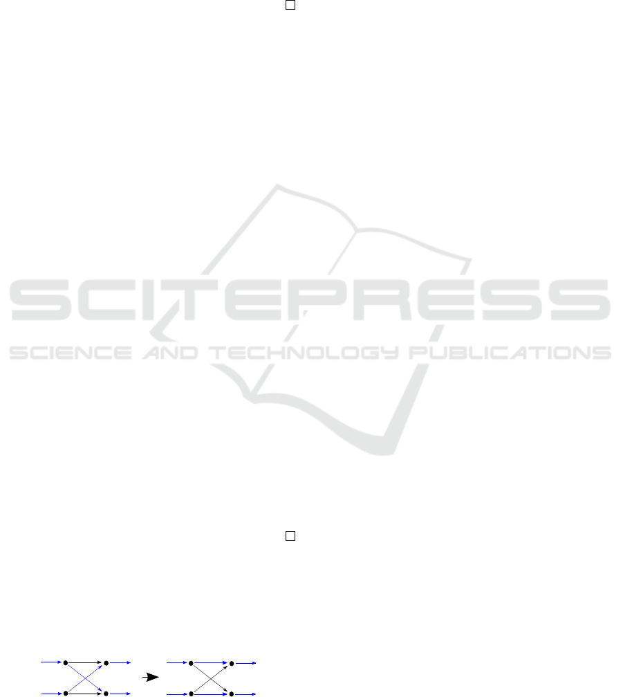
Theorem 2. The value of the flow heuristic is the
same when agents are allowed to swap in time ex-
panded graph as when swaps are forbidden.
Proof. The single-commodity flow anonymize both
goals and agents. Therefore, every agent is inter-
changeable with any other. When the heuristic plans
paths that make two agents swap their positions, it is
equivalent to path, where both agents stay in the same
position. If we found a time expanded graph with
minimal number of layers with desired flow, where
two agents swap, we can find equivalent flow, where
these two agents stay in the same position instead.
Such correction can be seen in Figure 4.
It is important to remember that the heuristic gives
us only numerical value, not the planned paths. We
introduce the correction of the paths only to show
that these paths are equivalent and the heuristic, as
described, gives sames results on any type of graph.
u'
j
v'
j
v
j+1
u
j+1
u'
j
v'
j
v
j+1
u
j+1
Figure 4: A correction of paths for anonymized agents on
undirected graph.
5 EXPERIMENT
We performed experimental comparison of the men-
tioned search-based techniques. Altogether we com-
pare four combinations of techniques, where the basic
for all of them is OD. The list of the combinations:
• OD with the baseline heuristic (OD+baseline)
• OD with the flow heuristic (OD+flow)
• OD+baseline with ID (OD+ID+baseline)
• OD+flow with ID (OD+ID+flow)
The experiments were conducted over two types
of graphs. The first one is a grid map 7x7 with obsta-
cles in the middle. This type of graph was selected for
its simple representation. The obstacles in the middle
of the graph are there to ensure high interaction be-
tween agents. This is further influenced by the start-
ing positions of the agents and their goal positions.
The goal positions are always in one cluster. The
starting positions are either in a cluster or in random
places. This will be further referenced as centered and
scattered respectively.
Since the algorithms are designed to work with
any type of graph, we also added randomized ori-
ented strongly biconnected graphs as a second type of
graph. We chose this type of graph because it is guar-
anteed to have solution, if there are at least two unoc-
cupied nodes (Botea and Surynek, 2015). For these
graphs, both starting and goal positions are random-
ized. Therefore there are three sets of test instances.
For all of these instances, we create differently dif-
ficult problems by increasing the number of agents
from 2 up to 12 agents. Each type of problem (i.e.
graph, starting positions, number of agents) is created
multiple times. When testing, we are interested in two
values. The total number of visited states - this is the
exact number of how many times a heuristic is com-
puted. The second value is the elapsed time during
computation. For each instance of problem, there is
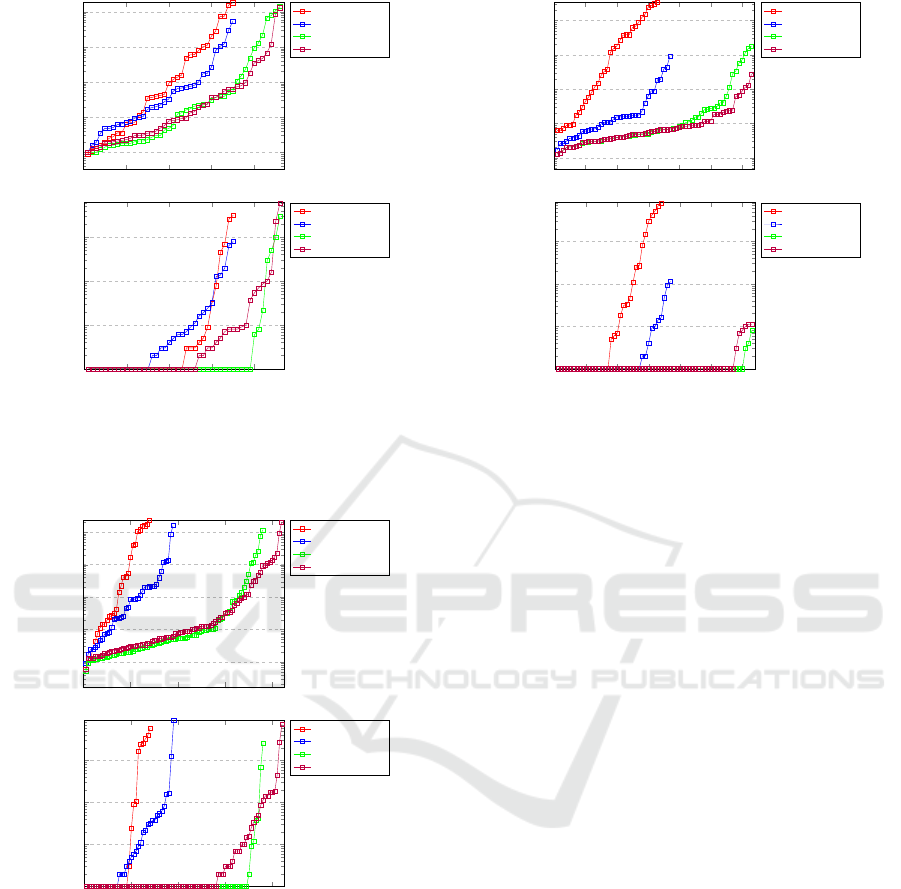
two minute timeout. In the following graphs, only in-
stances solved within the time limit are included. All
of the following graphs have a logarithmic y-axis to
better show differences even in smaller instances.
The fist type is grid graph with centered starting
positions (see Figure 5). These instances enforce high
interaction between agents, since they have to pass
through the small gap as a group. This is the rea-
son why adding ID does not improve the measured
values as much as in other instances. We can see
that the OD+flow outperforms OD+baseline in both
visited states and elapsed time. The other pair with
added ID performs similarly in terms of visited states.
In terms of computation time, the flow heuristic is
slightly worse since one call of the heuristic is more
difficult to compute than the baseline heuristic.
ICAART 2017 - 9th International Conference on Agents and Artificial Intelligence
456

0 10 20 30 40
10
1
10
2
10
3
10
4
10
5
Instance number
Number of visited states
Grid - centered
OD+baseline
OD+flow
OD+ID+baseline
OD+ID+flow
0 10 20 30 40
10
−2
10
−1
10
0
10
1
Instance number
Elapsed time [s]
OD+baseline
OD+flow
OD+ID+baseline
OD+ID+flow
Figure 5: Results of experiments on 7x7 grid with obstacles
and clustered starting positions. Top graph shows visited
states for ordered instances. Bottom graph shows computa-
tional time.
0 20 40
60
80
10
1
10
2
10
3
10
4
10
5
Instance number
Number of visited states
Grid - centered
OD+baseline
OD+flow
OD+ID+baseline
OD+ID+flow
0 20 40
60
80
10
−2
10
−1
10
0
10
1
Instance number
Elapsed time [s]
OD+baseline
OD+flow
OD+ID+baseline
OD+ID+flow
Figure 6: Results of experiments on 7x7 grid with obstacles
and randomized starting positions. Graphs are organized as
in Figure 5.
The second type is grid graph with random start-
ing positions (see Figure 6). These instances do not
enforce as high interaction between agents. This
means that ID is much more effective, as can be seen.
Both variants with flow heuristic outperforms their
counterparts in hard instances. For easier instances,
where the difference of searched states is much lower,
the easier heuristic outperforms flow heuristic in com-
putational time. In this example we can see that flow
heuristic is orthogonal improvement to ID.
0 10 20 30 40
50 60
10
1
10
2
10
3
10
4
10
5
Instance number
Number of visited states
Grid - centered
OD+baseline
OD+flow
OD+ID+baseline
OD+ID+flow
0 10 20 30 40
50 60
10
−2
10
−1
10
0
10
1
Instance number
Elapsed time [s]
OD+baseline
OD+flow
OD+ID+baseline
OD+ID+flow
Figure 7: Results of experiments on strongly biconnected
graph with randomized starting and goal positions. Graphs
are organized as in Figure 5.
The last type is randomized strongly biconnected
graph with randomized both starting and goal posi-
tions (see Figure 7). The results are similar to the
previous example with the same explanation.
6 DISCUSSION
We described a new heuristic for search-based algo-
rithms solving MAPF. The heuristic is based on net-
work flow over time expanded graph. The heuris-
tic was obtained as a relaxation of multi-commodity
flow, that can be used to solve MAPF, but is an NP-
hard problem. We showed that this heuristic is mono-
tone and therefore can be used effectively with search
algorithms. Further, we showed that this heuristic can
be used both for oriented and undirected graphs with
smaller construction of the time expanded graph than
is commonly used.
It can be noted that a single call of the flow heuris-
tic is harder to compute than other heuristics. If the
heuristic causes the search algorithm to expand less
states, it can still be beneficial to the overall comput-
ing time. However, in small instances where there is
not much room for improvement in terms of searched
states, the computational time may be worse. This
also affects usage of ID, since we start with smaller
groups of agents and thus easier problems. Future re-
search can focus on using both heuristic - the baseline
heuristic for instances with smaller number of agents
and the flow heuristic for instances with many agents.
New Flow-based Heuristic for Search Algorithms Solving Multi-agent Path Finding
457

ACKNOWLEDGEMENT
This paper is based on results obtained from SVV
project number 260 333, project commissioned by the
New Energy and Industrial Technology Development
Organization Japan, and the joint program for coop-
eration of the Israeli and Czech ministries of science
number 8G15027.
REFERENCES
Botea, A. and Surynek, P. (2015). Multi-agent path finding
on strongly biconnected digraphs. In Bonet, B. and
Koenig, S., editors, Proceedings of the Twenty-Ninth
AAAI Conference on Artificial Intelligence, January
25-30, 2015, Austin, Texas, USA., pages 2024–2030.
AAAI Press.
Boyarski, E., Felner, A., Stern, R., Sharon, G., Tolpin,
D., Betzalel, O., and Shimony, S. E. (2015). ICBS:
improved conflict-based search algorithm for multi-
agent pathfinding. In (Yang and Wooldridge, 2015),
pages 740–746.
Dinitz, E. (1970). Algorithm for solution of a problem of
maximal flow in a network with power estimation. So-
viet Math. Dokl., 11:1277–1280.
Even, S., Itai, A., and Shamir, A. (1976). On the complex-
ity of timetable and multicommodity flow problems.
SIAM J. Comput., 5(4):691–703.
Hart, P. E., Nilsson, N. J., and Raphael, B. (1968). A formal
basis for the heuristic determination of minimum cost
paths. IEEE Trans. Systems Science and Cybernetics,
4(2):100–107.
Kautz, H. A. and Selman, B. (1999). Unifying sat-based
and graph-based planning. In Dean, T., editor, Pro-
ceedings of the Sixteenth International Joint Confer-
ence on Artificial Intelligence, IJCAI 99, Stockholm,
Sweden, July 31 - August 6, 1999. 2 Volumes, 1450
pages, pages 318–325. Morgan Kaufmann.
Kornhauser, D., Miller, G. L., and Spirakis, P. G. (1984).
Coordinating pebble motion on graphs, the diame-
ter of permutation groups, and applications. In 25th
Annual Symposium on Foundations of Computer Sci-
ence, West Palm Beach, Florida, USA, 24-26 October
1984, pages 241–250. IEEE Computer Society.
Ma, H. and Koenig, S. (2016). Optimal target assignment
and path finding for teams of agents. In Proceedings
of the 2016 International Conference on Autonomous
Agents & Multiagent Systems, Singapore, May 9-13,
2016, pages 1144–1152.
Pearl, J. (1984). Heuristics - intelligent search strategies for
computer problem solving. Addison-Wesley series in
artificial intelligence. Addison-Wesley.
Ratner, D. and Warmuth, M. K. (1990). Nxn puzzle
and related relocation problem. J. Symb. Comput.,
10(2):111–138.
Ryan, M. R. K. (2008). Exploiting subgraph structure in
multi-robot path planning. J. Artif. Intell. Res. (JAIR),
31:497–542.
Sharon, G., Stern, R., Felner, A., and Sturtevant, N. R.
(2012). Conflict-based search for optimal multi-agent
path finding. In Hoffmann, J. and Selman, B., editors,
Proceedings of the Twenty-Sixth AAAI Conference on
Artificial Intelligence, July 22-26, 2012, Toronto, On-
tario, Canada. AAAI Press.
Sharon, G., Stern, R., Goldenberg, M., and Felner, A.
(2013). The increasing cost tree search for optimal
multi-agent pathfinding. Artif. Intell., 195:470–495.
Silver, D. (2005). Cooperative pathfinding. In Proceedings
of the First Artificial Intelligence and Interactive Digi-
tal Entertainment Conference, June 1-5, 2005, Marina
del Rey, California, USA, pages 117–122.
Standley, T. S. (2010). Finding optimal solutions to cooper-
ative pathfinding problems. In Fox, M. and Poole, D.,
editors, Proceedings of the Twenty-Fourth AAAI Con-
ference on Artificial Intelligence, AAAI 2010, Atlanta,
Georgia, USA, July 11-15, 2010. AAAI Press.
Surynek, P. (2009). A novel approach to path planning
for multiple robots in bi-connected graphs. In 2009
IEEE International Conference on Robotics and Au-
tomation, ICRA 2009, Kobe, Japan, May 12-17, 2009,
pages 3613–3619. IEEE.
Surynek, P. (2015). Reduced time-expansion graphs and
goal decomposition for solving cooperative path find-
ing sub-optimally. In (Yang and Wooldridge, 2015),
pages 1916–1922.
Yang, Q. and Wooldridge, M., editors (2015). Proceedings
of the Twenty-Fourth International Joint Conference
on Artificial Intelligence, IJCAI 2015, Buenos Aires,
Argentina, July 25-31, 2015. AAAI Press.
Yu, J. and LaValle, S. M. (2012). Multi-agent path plan-
ning and network flow. In Frazzoli, E., Lozano-P
´
erez,
T., Roy, N., and Rus, D., editors, Algorithmic Founda-
tions of Robotics X - Proceedings of the Tenth Work-
shop on the Algorithmic Foundations of Robotics,
WAFR 2012, MIT, Cambridge, Massachusetts, USA,
June 13-15 2012, volume 86 of Springer Tracts in Ad-
vanced Robotics, pages 157–173. Springer.
Yu, J. and LaValle, S. M. (2013a). Planning optimal paths
for multiple robots on graphs. In 2013 IEEE Interna-
tional Conference on Robotics and Automation, Karl-
sruhe, Germany, May 6-10, 2013, pages 3612–3617.
IEEE.
Yu, J. and LaValle, S. M. (2013b). Structure and intractabil-
ity of optimal multi-robot path planning on graphs. In
desJardins, M. and Littman, M. L., editors, Proceed-
ings of the Twenty-Seventh AAAI Conference on Arti-
ficial Intelligence, July 14-18, 2013, Bellevue, Wash-
ington, USA. AAAI Press.
ICAART 2017 - 9th International Conference on Agents and Artificial Intelligence
458