
Principles and Experiments of a Multi-Agent Approach for Large
Co-Simulation Networks Initialization
J
´
er
´
emy Boes, Tom Jorquera and Guy Camilleri
University of Toulouse, IRIT/Team SMAC, 118 route de Narbonne, Toulouse, France
Keywords:
Multi-Agent Systems, Self-Adaptive Systems, Co-Simulation.
Abstract:
Simulating large systems, such as smart grids, often requires to build a network of specific simulators. Making
heterogeneous simulators work together is a challenge in itself, but recent advances in the field of co-simulation
are providing answers. However, one key problem arises, and has not been sufficiently addressed: the initial-
ization of such networks. Many simulators need to have proper input values to start. But in the network, each
input is another simulator’s output. One has to find the initial input values of all simulators such as their com-
puted output is equal to the initial input value of the connected simulators. Given that simulators often contain
differential equations, this is hard to solve even with a small number of simulators, and nearly impossible with
a large number of them. In this paper, we present a mutli-agent system designed to solve the co-simulation
initialization problem, and show preliminary results on large networks.
1 INTRODUCTION
Alternatives to nuclear power, renewable energy like
solar panels or wind power, often involves producing
electricity near the consumers. This radically changes
the topology of the electric grid and makes it way
more difficult to manage and control. Smart grids are
a very active research field. Simulating smart grids
enables the validation of network control methods and
various network properties, that are as important as
the (simulated) physical properties of the power sys-
tem (Liberatore and Al-Hammouri, 2011). Neverthe-
less, designing a simulator and building a model for
large networks is a difficult task due to the complex-
ity of the considered systems. Co-simulation over-
comes this difficulty by running several models and
simulators together, one for each subsystem. In this
approach, simulators exchange data with each other,
in a ”black box” way. Models are then easier to ob-
tain since they only focus on a smaller part of the grid.
However, new problems arise, such as time synchro-
nization (Bouchhima et al., 2006). Most of them are
handled by existing co-simulation frameworks, but
the mutual and interdependent initialization of each
simulator is not.
Indeed, simulators in a co-simulation network re-
quire coherent initial values for their inputs. These in-
puts are connected to the outputs of other simulators.
To preserve the coherence in the network and prevent
simulators from crashing, the initial values that are set
have to be equal (or within a given accuracy limit) to
the values of the connected outputs of the other sim-
ulators. These output values are computed from the
other initial input values, that have been set under the
same constraints. Since each input is connected to an
output in the network, there is no ”first input” that is
free to go back to set an arbitrary value and solve the
whole problem.
Due to the large scale of co-simulations net-
works, the heterogeneity and the intrication of the
models involved, co-simulation initialization (or co-
initialization) is a difficult challenge. It requires a
lot of expertise and domain specific knowledge about
the models. Our approach aims at developping a co-
initialization method that does not rely on such exper-
tise, by considering each simulator as a black-box and
exploring the solutions. In this paper, co-initialization
is viewed as a fixed-point problem. We use a multi-
agent approach to find X such as F(X) = X, where F
is the function that transforms the inputs of all sim-
ulators into their outputs. The distributed and de-
centralised decision process of multi-agent systems
should allow our system to scale up to an increasing
number of simulators in the co-simulation network.
Section 2 presents the problem of co-initilization,
while our multi-agent system is described in section
3. Section 4 shows results before we conclude in the
last section.
58
Boes J., Jorquera T. and Camilleri G.
Principles and Experiments of a Multi-Agent Approach for Large Co-Simulation Networks Initialization.
DOI: 10.5220/0006186300580066
In Proceedings of the 9th International Conference on Agents and Artificial Intelligence (ICAART 2017), pages 58-66
ISBN: 978-989-758-219-6
Copyright
c
2017 by SCITEPRESS – Science and Technology Publications, Lda. All rights reserved

2 CO-INITIALIZATION
Co-initialization is the problem of finding adequate
initial values simultaneously for all the inputs of all
the simulators in a co-simulation network. This sec-
tion explains how we see this problem as a fixed-point
problem.
2.1 Co-Simulation
A co-simulation network is a network of possibly het-
erogeneous simulators running together to simulate
several parts or several scales of a large system. This
method enables to model huge systems that would be
otherwise too complex to handle with a single model,
and to reuse well-established and specialized model
with only minor modifications. For instance, to simu-
late an emergency brake maneuver for wind turbines,
Sicklinger et al. combine several models (blades,
gearbox, control system, etc) and achieve a more re-
alistic result than monolithic approaches (Sicklinger
et al., 2015).
Co-simulation has been of growing interest these
past years, but despite its efficiency, it does raise a
number of challenges. The development of a standard
for model exchange, called Functional Mock-up In-
terface (FMI), brings answers to the problem of mod-
els interoperability (Blochwitz et al., 2011). Other
tools deal with time coherence in co-simulation net-
works, such as MECSYCO which relies on the multi-
agent paradigm (Vaubourg et al., 2015).
2.2 Co-Initialization as a Fixed-Point
Problem
This paper addresses the issue of co-initialization, that
arises when simulators and models have constraints
on their input. For instance, some models can be un-
stable if their input changes too widely between two
timesteps, or crash if the inputs goes outside a given
range. In a co-simulation network, all simulators in-
puts are usually connected to an output from another
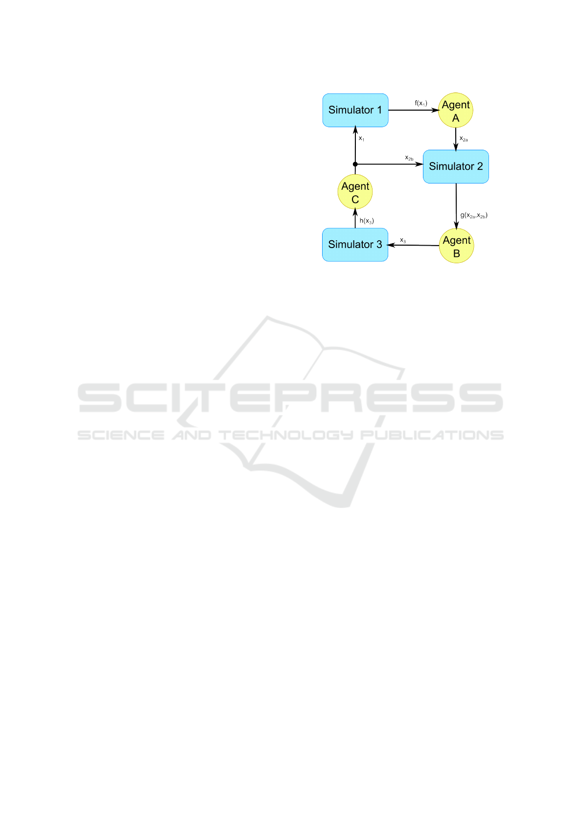
simulator. For instance, in figure 1, this means that
the initial value of the input of simulator 1 should be
equal or close to the output of simulator 3, which de-
pdends on the initial value of the input of simulator 3,
and so on with simulator 2.
If we consider simulators as functions, we can
express the co-initialization problem as a fixed-point
problem. For instance, with simulator 1 as function
f , simulator 2 function g, and simulator 3 function h,
the initialization problem is to find x
1
, x
2a
, x
2b
, and x
3
Figure 1: A Co-Simulation Network with 3 Simulators.
such as:
f (x
1
) = x
2a
g(x
2a
, x
2b
) = x
3
h(x
3
) = x
1
= x
2b
It is a fixed-point problem where we want to solve
X = F(X ) with X = (x
1
, x
2a
, x
2b
, x
3
) and F(X ) =
(h(x
3
), f (x
1
), h(x
3
), g(x
2a
, x
2b
)). In our case, we do
not know the models used by the simulators ( f , g, and
h are unknown). But we have access to their jacobian,
so we can know what variation would be caused on
an output by a modification of an input for a given
simulator.
2.3 Fixed-Point Solvers
The fixed-point problem is a challenging issue that
have many applications in fields where the notion
of stability can be expressed as a fixed-point, such
as economics and game theory (Border, 1989), pro-
gram analysis and code optimization (Costan et al.,
2005), or phase transition in physics (Schaefer and
Wambach, 2005).
The most common and proven approaches to solve
fixed-point problems are iterative methods (Alber
et al., 2003), (Yao et al., 2011). For instance, the
Newton-Raphson method (Bonnans et al., 2013) uses
the first terms of a Taylor series to approximate a
function for which we want to solve an equation.
While their formal definition is sound, this type of
approaches tends to suffer from combinatory explo-
sion when faced with a large number of dimensions.
This is why we work on an alternative solution with a
bottom-up multi-agent approach.
Principles and Experiments of a Multi-Agent Approach for Large Co-Simulation Networks Initialization
59
3 A SELF-ADAPTIVE
MULTI-AGENT SYSTEM FOR
CO-INITIALIZATION
This section details our multi-agent system and ex-
plains how agents help their neighborhood so the
whole system converge towards a solution.
3.1 Adapative Multi-Agent Systems
Our approach is inspired by the AMAS (Adaptive
Multi-Agent Systems) theory, a vision of multi-agent
systems where cooperation is the engine of self-
organization (Georg
´
e et al., 2011). The AMAS theory
is a basis for the design of multi-agent systems, where
cooperation drives local agents in a self-organizing
process which provides adaptiveness and learning
skills to the whole system. As cooperative entities,
AMAS agents seek to reach their own local goals as
well as they seek to help other agents achieving their
own local goals. Thus, an agent modifies its behavior
if it thinks that its actions are useless or detrimental to
its environment (including other agents).
The AMAS theory has proved useful and efficient
to tackle various problems where scaling up is a key
challenge, such as big data analytics (Belghache et al.,
2016), multi-satellite mission planning (Bonnet et al.,
2015), or air traffic simulation (Rantrua et al., 2015).
This is why we considered applying this approach to
the problem of large co-simulation initialization. The
system presented in this paper is homogeneous (all
agents have the same decision rules) and agents are
reactive, but it is not always the case with AMASs.
3.2 Agents Description
The key problem in co-simulation initialization lies in
the link between simulators. Thus, there is one agent
per link in the network, i.e. one agent for each out-
put of each simulator. In other words, there is only
one type of agent in our system, instanciated at each
output of each simulator.
3.2.1 Environment and Neighborhood
The environment of an agent is composed of all the
simulators and all the other agents. But agents per-
ceive their environment only partially. Each agent has
one input and one output. The value of its input is per-
ceived in the environment, it is the output of the cor-
responding simulator. The value of the agent’s output
is decided by the agent itself, on its own. This output
is connected to one or several simulators, depending
on the co-simulation network.
Figure 2: A Co-Simulation Network with 3 Simulators and
our Agents.
The neighborhood of an agent A is defined as the
agents that are directly affected by the output of agent
A, including itself. Hence, the neighborhood of agent
A is composed of agent A and all the agents at the
output of the simulators connected to the output of
agent A. For instance, in figure 2, the neighborhood
of agent A is composed of agent A and agent B.
The global goal of the system is to reach a state in
which each agent perceives on its input the same value
it had written on its output at the previous timestep.
This would mean the network is correctly initialized
since the computed outputs of the simulators are sta-
ble.
3.2.2 Criticality of an Agent
Each agent seeks to meet the condition |x
t
−y
t−1
| = 0,
where x is the input of the agent, y its output, and t the
timestep. It is a reformulation of the fixed point prob-
lem for the network, but centered on the links rather
than on the nodes. The value c = |x
t
− y
t−1
| is called
the criticality of the agent. The higher its critical-
ity, the less satisfied an agent is. We define C
sys
the
global criticality of the system as the highest critical-
ity among the agents. By definition, the problem is
solved when C
sys
= 0. It is a mere reformulation of
the fixed-point problem expressed in 2.2 that is more
suitable for our approach.
At each timestep, each agent computes its critical-
ity, watches the criticalities in its neighborhood, and
tries to correlate their variation to the variation of its
own output. The agents adjust their output value in
order to lower their neighbors’ criticality. The next
section explains how they decide their output value.
ICAART 2017 - 9th International Conference on Agents and Artificial Intelligence
60

3.3 Agents Behavior
Each agent has to decide its next action: whether to
increase or decrease its value, and by what amount,
in order to lower the criticality of its neighborhood as
quickly as possible. Its output y at timestep t is:
y
t
= y
t−1
+ a
t
Where a
t
is the decided action. The decision is based
on two dynamically adjusted internal variables:
• δ ∈ R
+
, with δ
min
≤ δ ≤ δ
max
is the amplitude of
the action, δ
min
and δ
max
are user-defined parame-
ters, which will be discussed later ;
• σ ∈ N with −n ≤ σ ≤ n indicates the sign of the
action, n is a user-defined parameter of the agent,
which will be discussed later.
These two variables directly define a:
a :=
(
δ ×
σ
|σ|
if σ 6= 0
random(−δ, δ) otherwise
The sign of σ is the sign of the action, and the abso-
lute value of σ reflects how much the agent is con-
vinced that the sign is correct. If σ = 0, the decision
is a coin flip between −δ and δ. We introduced ran-
domness here because all agents perceive and decide
simultaneously, thus falling into the El Farol bar prob-
lem (Whitehead, 2008).
3.3.1 Adaptation
Each agent dynamically manages its own internal δ
and σ variables, and decide how to adapt them. This
section explains how an agent adjusts its δ and σ.
Thanks to the jacobians provided by the simula-
tors connected on its output, the agent computes a
criticality jacobian, giving him an estimation of the
variations of the criticalities of its neighborhood. The
agent splits its neighbors into two groups, regarding
their criticality jacobian:
• the most critical group contains the most critical
neighbor (i.e. the neighbor with the highest crit-
icality) and all the neighbors whose criticality ja-
cobian has the same sign as the criticality jacobian
of the most critical neighbor. This means that if
the agent helps its most critical neighbor, its ac-
tion will also help all the other neighbors of this
group.
• the opposite group contains all the neighbors
whose criticality jacobian are of opposite sign
with the criticality jacobian of the most critical
neighbor. This means that if the agent helps its
most critical neighbor, its action will aslo hurt all
the neighbors of this group.
We call worst neighbor the most critical neighbor,
and opposite worst neighbor the most critical neigh-
bor from the opposite group. The goal for the agent
is then to help its worst neighbor while preventing its
opposite worst neighbor to become the worst neigh-
bor.
The agent observes four indicators in its environ-
ment to decide how to adjust its δ and σ:
• the direction of variation of the criticality of its
worst neighbor,
• the direction of variation of the criticality of its
opposite worst neighbor,
• the direction of variation of the difference be-
tween the worst neighbor’s criticality and the op-
posite worst neighbor’s criticality,
• the correlation between the sign of σ and the sign
of the criticality jacobian of the worst neighbor,
which indicates if the action of the agent is cur-
rently helping the worst neighbor or the opposite
worst neighbor.
Before computing its action, the agent adapts its δ
and σ according to a small set of rules conditioned
by these four indicators. These rules are presented in
table 1.
”Strengthen σ” means its absolute value is in-
creased without changing its sign: if σ is positive then
σ is incremented by one (decremented by one other-
wise). Likewise, ”weaken σ” means its absolute value
of σ is decreased without changing its sign: if σ is
positive then σ is decremented by one (incremented
by one otherwise). Finally, ”increase δ” means δ is
multiplied by α > 1 and ”decrease δ” means it is di-
vided by β > 1. α and β are user-defined parameters.
The idea underlying this set of rules is to decrease
as fast as possible the criticality of all the neighbors.
The agent seeks to maximize its δ while reducing the
difference between the criticality of the worst neigh-
bor and the criticality of the opposite worst neighbor.
The worst case for an agent is when the condi-
tions of line 1 occur: the criticality of both the worst
neighbor and the opposite worst neighbor are increas-
ing, the highest criticality faster than the other. In
this case, the agent adjusts σ and δ in order to give
more help to its worst neighbor and less to the oppo-
site worst neighbor.
The best case is in line 8, when the criticality of
both the worst neighbor and the opposite worst neigh-
bor are decreasing, and the highest criticality is de-
creasing faster. This is an ideal situation if σ = n or
σ = −n, meaning that the agent is certain about its
current action.
Principles and Experiments of a Multi-Agent Approach for Large Co-Simulation Networks Initialization
61
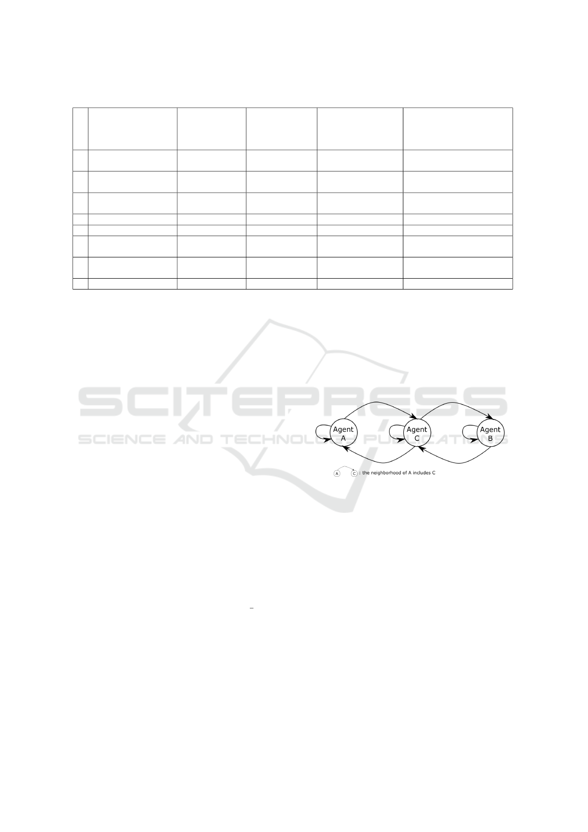
Table 1: Rules of Adaptation.
#
Variation
of the criticality
of the worst neighbor
Variation
of the criticality
of the opposite
worst neighbor
Variation
of the difference
between these
two neighbors
Decision of an agent
currently helping
its worst neighbor
Decision of an agent
currently helping
its opposite worst neighbor
1 ↑ ↑ ↑
strengthen σ,
increase δ
weaken σ,
decrease δ
2 ↑ ↑ ↓ decrease δ
weaken σ,
decrease δ
3 ↑ ↓ ↑
strengthen σ,
increase δ
weaken σ,
decrease δ
4 ↑ ↓ ↓
impossible impossible
5 ↓ ↑ ↑ impossible impossible
6 ↓ ↑ ↓ strengthen σ
strengthen σ,
increase δ
7 ↓ ↓ ↑
strengthen σ,
increase δ
strengthen σ,
decrease δ
8 ↓ ↓ ↓ strengthen σ strengthen σ
3.3.2 Parameters
There are six parameters for the agents:
• n - defines the boundaries of σ, that varies be-
tween −n and n.
• δ
init
- since δ is adjusted in real time, the system
is able to converge for any initial value of δ but a
proper δ
init
may help for a quicker convergence.
• δ
min
- the minimal value for δ has to be strictly
positive, because δ
min
= 0 often leads to dead-
locks.
• δ
max
- the maximal value for δ is merely a safety
guard to avoid too big variations. If δ
min
= δ
max
the system works with a constant δ.
• α - the ”increase factor” by which δ is multiplied
when it needs to increase,
• β - the ”decrease factor” by which δ is divided
when it needs to decrease.
α and β both have to be strictly greater than one. They
are the only really sensitive parameters as the stabi-
lization of the system depends on them. α should be
small comparatively to β. Although a thorough study
of their impact is needed, in our experiments we never
had good results when α was greater than
1
2
β. For
some experiments, the best results were obtained with
β worths 100 times α.
Generally, the lower δ
min
and δ
max
the more pre-
cise the solution, but at the cost of more timesteps to
reach it. A greater β makes δ more frequently close
to δ
min
, hence gaining precision and loosing speed of
convergence, and vice versa for α. A big α tends to
harm the stability of the system, provoking big oscil-
lations around the solution instead of smoothly con-
verging towards it. Finally, n impacts the inertia of
the system: if it is high, an agent will be slower to
change direction after having strengthened σ several
times consecutively.
Except for δ
init
all the parameters can be interac-
tively modified at runtime, the system will self-adapt
according to the new values.
Figure 3: Neighborhood Graph of a 3 Nodes Test Case.
4 RESULTS
This section shows results of various experiments
on generated networks with polynomial nodes. We
used a generator to create random topologies of net-
works of polynomial nodes. Nodes are of the form of
ax
2
+ bx + c with random a, b and c. For these ex-
periments, our system is implemented in Java 1.7 and
runs on an HP Elitebook laptop with an Intel Core i7
processor and 16GB of RAM. The parameters were
set as follows:
• n = 3
• δ
init
= 1.0
• δ
min
= 0.001
• δ
max
= 1.0
ICAART 2017 - 9th International Conference on Agents and Artificial Intelligence
62
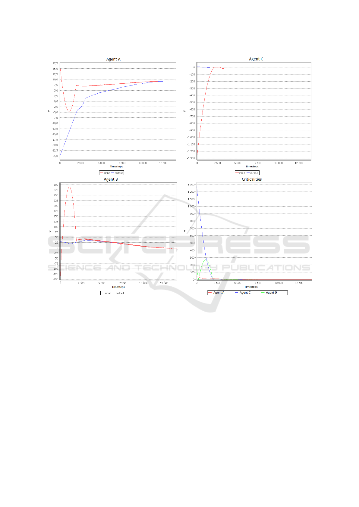
Figure 4: Convergence with a 3 Nodes Network.
• α = 1.2
• β = 100
These values were obtained empirically through ex-
tensive testing and proved to be efficient for all our ex-
perimentations with networks of second degree poly-
nomial nodes, regardless of the topology.
4.1 3 Polynomial Nodes
Our first experiment involves a simple 3 nodes net-
work. Figure 3 shows the neighborhood graph of this
simple case. It is a representation of the network of in-
fluence of the agents. An edge from A to B means that
the neighborhood of A includes B, in other words A
directly impacts B via a simulator. Here agent A has
two neighbors including itself, agent B has two neigh-
bors including itself, and agent C has three neighbors
including itself.
Figure 4 shows the input and output of each agent
during the resolution, along with their criticalities (the
difference between their input and their output). We
see that at the beginning, the most critical agent is
C. Since it is in the neighborhood of both A and B,
these agents tend to help C more, even if it increases
their own criticality. Around timestep 1500, agent B
is on the verge to become the most critical agent. The
agents (including B itself) react and find a way to de-
crease both C and B’s criticalities, at the expense of
A. In the end, they all have converged toward a stable
state where their criticality is less than δ
min
(presently
10
−3
). It took approximatively 10000 timesteps (3
seconds).
Principles and Experiments of a Multi-Agent Approach for Large Co-Simulation Networks Initialization
63
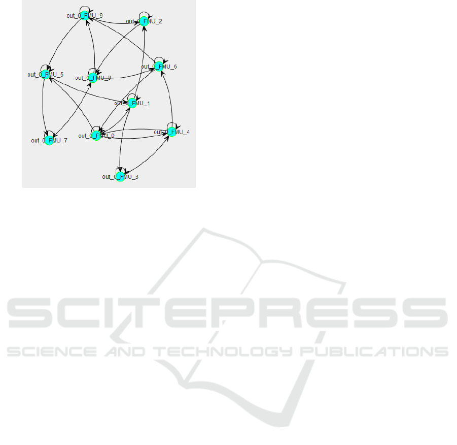
Figure 5: Neighborhood Graph of a 10 Nodes Test Case.
4.2 10 Polynomial Nodes
In this experiment, we test our system with a bigger
network. Figure 5 shows the neighborhood graph of
our MAS for this case. For the sake of concision and
readability, we do not show here the input and output
curves of each agents, but only their criticalities (6).
We can see that the agents immediately find a way
to decrease the worst criticalities, but then struggle
to make the residual criticalities disappear. However,
they end up finding a way to reach a state where each
criticality is less than δ
min
. It took approximatively
14000 timesteps (30 seconds).
With the same parameters, for a network more
than three times the size of the previous one, the num-
ber of timesteps to converge is only 40% greater than
the previous case. Unfortunately, the duration is about
7 times longer.
4.3 100 Polynomial Nodes
This experiments show how the MAS scales up to a
network of 100 polynomial nodes. We do not present
the neighborhood graph because it is unreadable. Fig-
ure 7 shows the criticalities of all agents. We see that
the systems converge in about 18500 timesteps. This
is only 1.32 times more timesteps, while the network
is ten time bigger. However, this time the computa-
tion took 90 minutes to complete (180 times longer
than the 10 nodes network).
4.4 Discussion
The main result of these experiments is that the num-
ber of timesteps to find a solution does not increase
with the size of the network. In other words, the sys-
tem scales up to the size of the network in term of
the the total number of actions needed for each agent.
However, the duration of the computation increases
with the size of the network. This is mainly due to the
fact that our prototype is single-threaded: the compu-
tation of each node has to be done sequentially. Co-
simulations can be distributed, sometimes even phys-
ically distributed, enabling to compute each node of
the network in parallel. Moreover, our agents take
completely local decisions and do not need sophisti-
cated synchronization. This is why our future work
will focus on the parallelization of our implementa-
tion. This should significantly improve time of com-
putation, making the system also scalable in terms of
duration of computation.
5 CONCLUSION AND FUTURE
WORKS
Co-initialization, the problem of properly initializ-
ing interdependent simulators in a co-simulation is
challenging, especially when simulators are numer-
ous. This problem can be reinterpreted as a fixed-
point problem, for which current methods suffer from
a lack of scalability. This paper presented a multi-
agent approach where each output of each simula-
tor is an agent trying to find an initial value for the
simulators that are connected to it. Agents seek to
help their neighborhood as well as themselves, and
together converge towards a stable solution.
Results show that this approach is efficient and
scales up to the number of simulators regarding the
number of timesteps required to reach a solution. It
takes only 1.85 times more timesteps to initialize a
network of 100 simulators than a network of 3 sim-
ulators. However, our current single-threaded Java
implementation does not scale: because their execu-
tion is sequential, the higher the number of simula-
tors, the longer a timestep is. Future work will fo-
cus on a multi-threaded parallelized implementation
to make the system also scalable in terms duration of
computation. Our intention is also to get rid of the
jacobians. The less the agents need to know about the
models, the more generic our approach will be. This
could be achieved by enhancing the learning abilities
of the agents, so they improve their understanding of
the simulators with each action they make. Finally, a
better formalization of the system and a more theoret-
ical analysis are needed before moving forward with
extensive comparisons with other fixed-point solvers.
ICAART 2017 - 9th International Conference on Agents and Artificial Intelligence
64
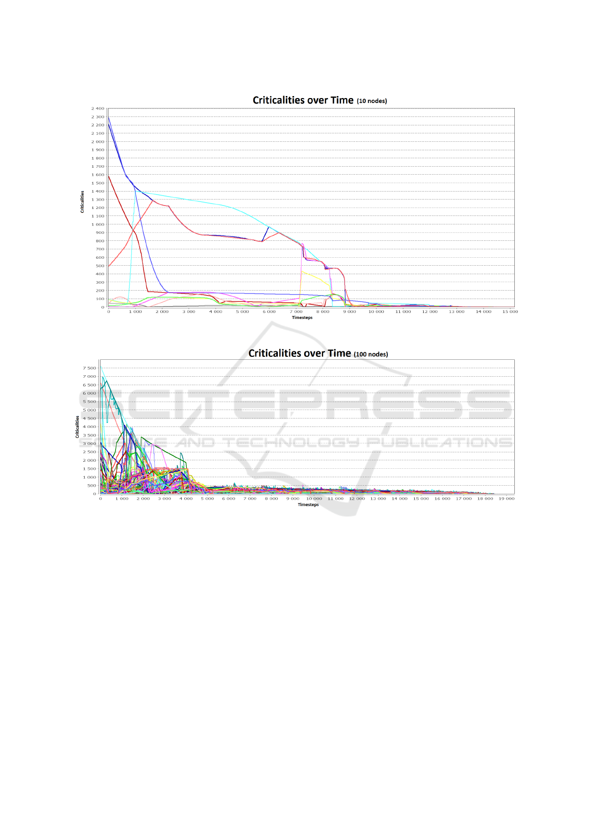
Figure 6: Convergence with a 10 Nodes Network.
Figure 7: Convergence with a 100 Nodes Network.
REFERENCES
Alber, Y., Reich, S., and Yao, J.-C. (2003). Iterative meth-
ods for solving fixed-point problems with nonself-
mappings in banach spaces. Abstract and Applied
Analysis, 2003(4):193–216.
Belghache, E., Georg
´
e, J.-P., and Gleizes, M.-P. (2016). To-
wards an Adaptive Multi-Agent System for Dynamic
Big Data Analytics. In The IEEE International Con-
ference on Cloud and Big Data Computing (CBD-
Com), Toulouse, France. IEEE Computer Society -
Conference Publishing Services.
Blochwitz, T., Otter, M., Arnold, M., Bausch, C., Clauß, C.,
Elmqvist, H., Junghanns, A., Mauss, J., Monteiro, M.,
Neidhold, T., et al. (2011). The functional mockup
interface for tool independent exchange of simulation
models. In 8th International Modelica Conference,
pages 105–114, Dresden.
Bonnans, J.-F., Gilbert, J. C., Lemar
´
echal, C., and Sagas-
tiz
´
abal, C. A. (2013). Numerical optimization: the-
oretical and practical aspects. Springer Science &
Business Media.
Bonnet, J., Gleizes, M.-P., Kaddoum, E., Rainjonneau, S.,
and Flandin, G. (2015). Multi-satellite mission plan-
ning using a self-adaptive multi-agent system. In
IEEE International Conference on Self-Adaptive and
Self-Organizing Systems (SASO), Cambridge, MA,
USA, pages 11–20. IEEE Computer Society - Confer-
ence Publishing Services.
Border, K. C. (1989). Fixed point theorems with applica-
tions to economics and game theory. Cambridge Uni-
versity Press.
Principles and Experiments of a Multi-Agent Approach for Large Co-Simulation Networks Initialization
65

Bouchhima, F., Briere, M., Nicolescu, G., Abid, M., and
Aboulhamid, E. M. (2006). A systemc/simulink co-
simulation framework for continuous/discrete-events
simulation. In Behavioral Modeling and Simulation
Workshop, Proceedings of the 2006 IEEE Interna-
tional, pages 1–6.
Costan, A., Gaubert, S., Goubault, E., Martel, M., and
Putot, S. (2005). A policy iteration algorithm for
computing fixed points in static analysis of programs.
In Etessami, K. and Rajamani, S. K., editors, Com-
puter Aided Verification: 17th International Confer-
ence, CAV 2005, Edinburgh, Scotland, UK, July 6-10,
2005. Proceedings, pages 462–475. Springer Berlin
Heidelberg, Berlin, Heidelberg.
Georg
´
e, J.-P., Gleizes, M.-P., and Camps, V. (2011). Co-
operation. In Di Marzo Serugendo, G., Gleizes,
M.-P., and Karageogos, A., editors, Self-organising
Software, Natural Computing Series, pages 7–32.
Springer Berlin Heidelberg.
Liberatore, V. and Al-Hammouri, A. (2011). Smart grid
communication and co-simulation. In Energytech,
2011 IEEE, pages 1–5.
Rantrua, A., Maesen, E., Chabrier, S., and Gleizes, M.-P.
(2015). Learning Aircraft Behavior from Real Air
Traffic. The Journal of Air Traffic Control, 57(4):10–
14.
Schaefer, B.-J. and Wambach, J. (2005). The phase dia-
gram of the quark–meson model. Nuclear Physics A,
757(3):479–492.
Sicklinger, S., Lerch, C., W
¨
uchner, R., and Bletzinger, K.-
U. (2015). Fully coupled co-simulation of a wind
turbine emergency brake maneuver. Journal of Wind
Engineering and Industrial Aerodynamics, 144:134–
145.
Vaubourg, J., Presse, Y., Camus, B., Bourjot, C., Ciar-
letta, L., Chevrier, V., Tavella, J.-P., and Morais, H.
(2015). Multi-agent multi-model simulation of smart
grids in the ms4sg project. In International Confer-
ence on Practical Applications of Agents and Multi-
Agent Systems (PAAMS 2015), pages 240–251, Sala-
manca, Spain. Springer.
Whitehead, D. (2008). The el farol bar problem revisited:
Reinforcement learning in a potential game. ESE Dis-
cussion Papers, 186.
Yao, Y., Cho, Y. J., and Liou, Y.-C. (2011). Algorithms
of common solutions for variational inclusions, mixed
equilibrium problems and fixed point problems. Eu-
ropean Journal of Operational Research, 212(2):242
– 250.
ICAART 2017 - 9th International Conference on Agents and Artificial Intelligence
66
