Estimating Coarse 3D Shape and Pose from the Bounding Contour

Paria Mehrani and James H. Elder

Department of Electrical Engineering and Computer Science, York University, 4700 Keele Street, Toronto, Canada

paria@cse.yorku.ca, jelder@yorku.ca

Keywords:

Shape Estimation, 3D Shape Reconstruction, Single-view Reconstruction, Shape-from-contour.

Abstract:

Single-view reconstruction of a smooth 3D object is an ill-posed problem. Surface cues such as shading and

texture provide local constraints on shape, but these cues can be weak, making it a challenge to recover globally

correct models. The bounding contour can play an important role in constraining this global integration. Here

we focus in particular on information afforded by the overall elongation (aspect ratio) of the bounding contour.

We hypothesize that the tendency of objects to be relatively compact and the generic view assumption together

induce a statistical dependency between the observed elongation of the object boundary and the coarse 3D

shape of the solid object, a dependency that could potentially be exploited by single-view methods. To test

this hypothesis we assemble a new dataset of solid 3D shapes and study the joint statistics of ellipsoidal

approximations to these shapes and elliptical approximations of their orthographically projected boundaries.

Optimal estimators derived from these statistics conﬁrm our hypothesis, and we show that these estimators

can be used to generate coarse 3D shape-pose estimates from the bounding contour that are signiﬁcantly and

substantially superior to competing methods.

1 INTRODUCTION

To be clear on terminology, we follow (Koenderink,

1984) and refer to the set of surface points grazed by

the view vector as the rim of the object, and the pro-

jection of these points into the image as the occluding

contour.

It is well known that the occluding contour

strongly constrains surface shape at the rim (Koen-

derink, 1984). Indeed, human judgement of sur-

face shape is strongly inﬂuenced by the shape of the

occluding contour (Todd and Reichel, 1989; Todd,

2004), and often even the occluding contour alone

provides a compelling sense of volumetric shape (Tse,

2002; Elder, 2014) (Fig. 1). Understanding the infor-

Figure 1: Volumetric shape from the bounding contour.

mation provided by the occluding contour is impor-

tant not only for this limiting case, but also for devis-

ing algorithms that effectively exploit contour cues in

conjunction with (possibly weak) surface cues such as

shading and texture (Karsch et al., 2013).

While the computer vision literature on shape

from contour is relatively small, there have been a

few interesting studies in recent years exploring the

degree to which solid shape can be reconstructed

from occluding contours alone (Igarashi et al., 1999;

Twarog et al., 2012; Karsch et al., 2013). These stud-

ies have tended to focus on extracting a complete, de-

tailed model of the 3D shape from the boundary, with-

out considering whether the solution will be close to

correct at a global scale. Here we take the opposite

view, and ask whether the bounding contour can tell

us anything about the global shape of the object at the

coarsest scale and its 3D pose. If this global informa-

tion can be estimated from the bounding contour, it

could then be used to help constrain algorithms that

recover more detailed 3D structure so that reconstruc-

tions are correct at both local and global scales.

Most computer vision work in this area exploits

the bounding contour in conjunction with surface cues

within an optimization framework. Typically, user in-

teraction and/or some inﬂation term in the objective

function are required to avoid a trivial (ﬂat) solution.

Users were required to specify depth of some sur-

face points in (Prasad et al., 2006), or a ﬁxed volume

that the shape must ﬁll in (Toppe et al., 2011). Os-

wald (Oswald et al., 2009) used an inﬂation term.

More recent studies has avoided user interaction

Mehrani P. and Elder J.

Estimating Coarse 3D Shape and Pose from the Bounding Contour.

DOI: 10.5220/0006190306030610

In Proceedings of the 12th International Joint Conference on Computer Vision, Imaging and Computer Graphics Theory and Applications (VISIGRAPP 2017), pages 603-610

ISBN: 978-989-758-225-7

603

and arbitrary inﬂation terms and instead have com-

bined local surface shading cues with contour infor-

mation to estimate surface shape. Cole (Cole et al.,

2012) estimate local surface normals within an MRF

framework and ﬁt a ﬁnal 3D surface to the estimated

normals using a thin plate spline. Barron and Ma-

lik (Barron and Malik, 2015) assume a probabilis-

tic framework, imposing a prior over the variation in

mean surface curvature. While both of these systems

fuse shading and contour cues to determine the re-

construction, Karsch (Karsch et al., 2013) have shown

that internal contour cues appear to be stronger cues

to shape than shading.

A very different strategy for single-view es-

timation of smooth solid shapes was ﬁrst intro-

duced in the interactive sketching interface dubbed

Teddy (Igarashi et al., 1999) and later studied by

Twarog (Twarog et al., 2012) under the pseudonym

Puffball. (We will use the latter term as an evocative

label for this class of methods.) In this approach, the

solid shape is deﬁned as the envelope of spheres cen-

tred on the interior skeleton (Blum, 1973) of the shape

in the image, and bi-tangent to the occluding contour

(Fig. 2). The method is simple and can produce sur-

prisingly reasonable results in many cases.

Figure 2: Puffball reconstruction (Twarog et al., 2012).

One limitation of all of these prior algorithms is

that they are typically constrained or at least strongly

biased to return a planar or near-planar and fronto-

parallel rim (i.e., a frontal pose), whereas in the real

world under general viewing the probability of this is

vanishing. A second potential problem is that these

methods impose strong constraints or priors on the

overall depth of the objects. For example, by deﬁn-

ing solid shape as an envelope of spheres, Puffball

makes a very strong local symmetry assumption: at

every point on the skeleton, the depth of the object

(dimension in the viewing direction) is equal to twice

the distance of the contour from the skeleton. Are

these assumptions reasonable?

One of the difﬁculties in answering this question

is that most prior work has been evaluated only qual-

itatively, not quantitatively. Important exceptions are

the work of Karsch (Karsch et al., 2013) and Barron &

Malik (Barron and Malik, 2015), however their eval-

uations do not explicitly test these assumptions.

2 OUR CONTRIBUTIONS

Instead of focusing on detailed shape reconstruction,

our goal in this paper is to understand information af-

forded by the bounding contour on the rough shape

and global 3D pose of the object. In particular, we

wish to understand whether the contour can provide a

cue to the rough length, width and depth of the object,

and how it might be angled out of the fronto-parallel

plane. To address this question we will study the

joint statistics of ellipsoidal approximations of real

scanned objects and their image projections. Here

we conﬁne ourselves to orthographic projection, un-

der which these ellipsoidal approximations generate

elliptical images.

Our speciﬁc contributions are:

1. We introduce a new dataset and methodology for

evaluating methods for single-view reconstruction

of smooth solid objects.

2. We show that statistically, even a simple elliptical

approximation of the occluding contour provides

substantial information about the coarse 3D shape

and pose of the object.

3. We show that the assumptions of symmetry in

depth and fronto-parallel pose imposed by prior

work lead to large errors in single-view 3D object

estimation.

3 INTUITION

Why would a simple elliptical approximation to the

occluding contour carry information about 3D shape

and pose? One of our intuitions is rooted in the com-

pactness of real objects. While objects vary widely

in shape, we conjecture that extreme elongations are

relatively rare. This has implications when we ob-

serve an elongated occluding contour in the image

(Fig. 3(a)).

There is an inﬁnite family of solid objects that

could have generated this contour. However, if the

longest dimension of the object is angled away from

fronto-parallel, the object must be even more elon-

gated than the occluding contour. This induces a bias

for elongated occluding contours to project from ob-

jects whose long dimension is close to fronto-parallel,

whereas for less elongated contours the long dimen-

sion is relatively more likely to be angled away from

the image plane.

A second intuition derives from the generic view-

point assumption (Freeman, 1994). Imagine an elon-

gated object with its longest dimension in the view-

ing direction (Fig. 3(b)). A small change in 3D pose

VISAPP 2017 - International Conference on Computer Vision Theory and Applications

604

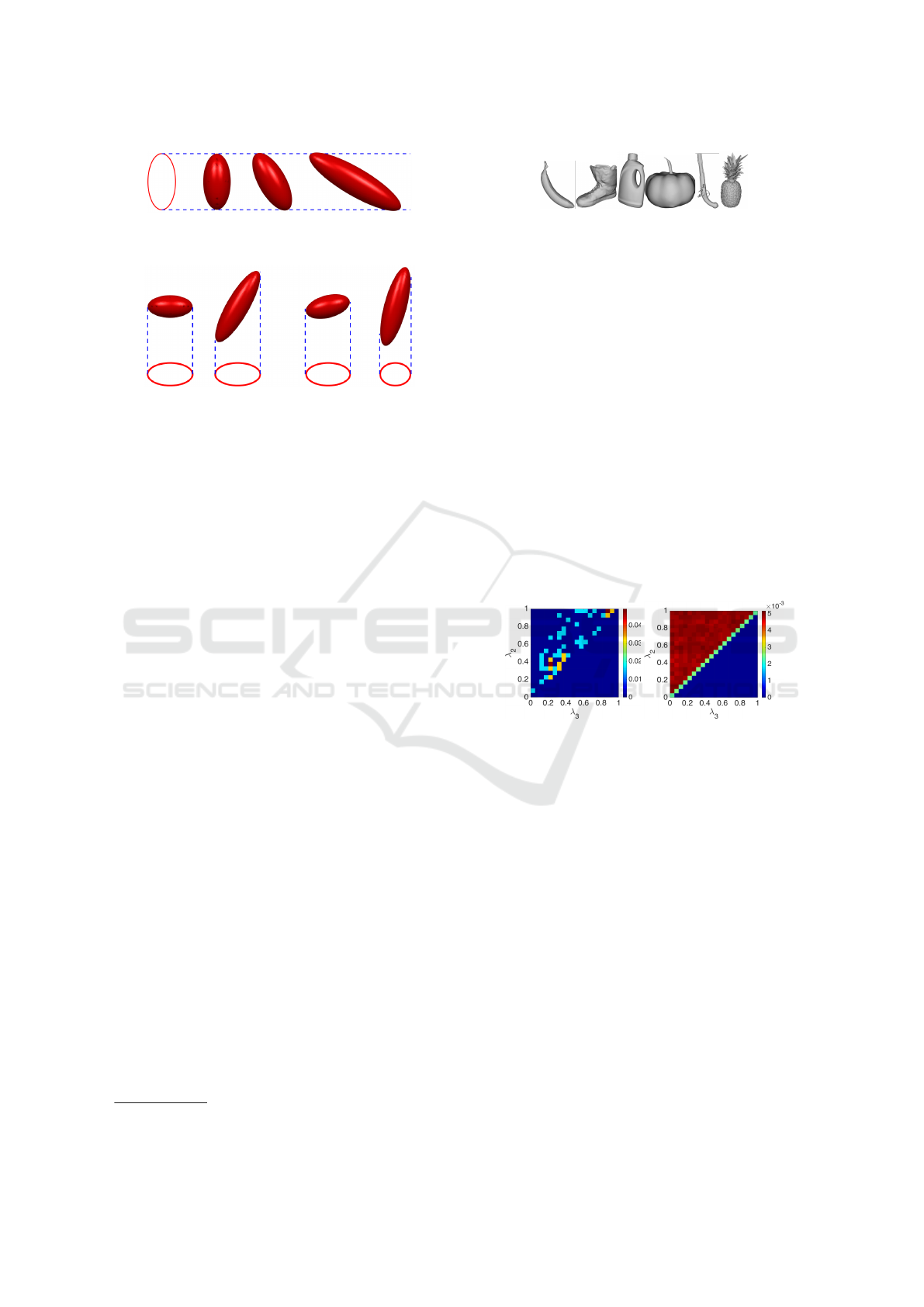
(a) Ellipsoids of various shapes can give rise to

the same ellipse. The ellipse is viewed from

front while ellipsoids are viewed from top.

(b) Two ellipsoids giving rise to the same ellipse

with and without fronto-parallel poses (left), and

same ellipsoids rotated 15 deg. The projection

of the longer ellipsoids has drastic changes with

small perturbations in pose (right).

Figure 3: Top: An inﬁnite family of shapes can project onto

the same contour. Bottom: Drastic changes in projection of

an elongated ellipsoid with small perturbations in its pose.

will induce a large change in the appearance of the

occluding contour. If, on the other hand, the object is

rotated so that its smallest dimension is in the viewing

direction, the same change in 3D pose will induce a

relatively small change in the occluding contour. This

suggests that the expected extent of the object in depth

may be small relative to the dimensions observed in

the image, counter to the Puffball assumption.

These are only qualitative intuitions. The main

point of this paper is test these intuitions quantita-

tively, using a simple sampling technique.

4 DATASET

At time of writing, we are not aware of any large-scale

public collection of real 3D scanned objects. For the

purposes of this project, we have therefore assembled

a collection from various sources on the internet in-

cluding the BigBIRD dataset (Singh et al., 2014), the

YCB object and model set dataset (C¸ alli et al., 2015),

and various other 3D model sharing websites such as

Sketchfab

. Any duplicates were removed. The ﬁnal

dataset consists of 122 objects, which we randomly

divided into training and test sets of 61 objects each.

Some examples are shown in Fig. 4.

https://sketchfab.com.

Figure 4: Example 3D objects in our dataset.

5 METHODS

5.1 Priors

We employ ellipsoids as low-order 3D models cap-

turing global shape and pose. We ﬁrst use an iterative

closest point algorithm (Besl and McKay, 1992) to

determine, for each object in the dataset, the ellipsoid

that minimizes mean squared Euclidean error (Fig-

ures 12 and 13). The size and shape of each ellipsoid

is completely characterized by the length of its three

axes: a ≥ b ≥ c. Since we are not concerned with ab-

solute size, we can collapse these three numbers into

two ratios specifying the length of its two smaller axes

relative to the largest axis: 1 > λ

= b/a > λ

= c/a >

0 . The collection of ellipsoid ﬁts to our training data

then form our empirical shape prior (Fig. 6(a)).

Figure 5: Ellipsoid shape priors. Left: Empirical prior de-

rived from training objects. Right: Theoretical prior, based

on a uniform distribution of axis lengths.

There are two major limitations of this prior. First,

given the limited size of our dataset, it is of course

quite noisy. Second, since we employed opportunity

sampling to form the dataset, it is certain to contain

bias. For these reasons, we also constructed a theoret-

ical uniform shape prior, formed by sampling triplets

of numbers uniformly on [0, 1], scaling each triplet to

have maximum value 1, and then assigning the middle

and smaller values to b and c. As expected, the result-

ing distribution is uniform on the subspace λ

≥ λ

(The green diagonal stripe reﬂects the fact that only

half of each bin on the diagonal lies in the feasible

subspace.) Note that the mean of this distribution is

(λ

= 2/3,λ

= 1/3). In other words, the mean shape

under the uniform prior has axes in the ratio 3 : 2 : 1.

While the limited sample size for the empirical

prior makes detailed comparison with the uniform

prior difﬁcult, we can at least make some qualita-

tive observations. First, the empirical prior seems to

Estimating Coarse 3D Shape and Pose from the Bounding Contour

605

be biased somewhat toward more compact, less elon-

gated ellipsoids, i.e., toward λ

= λ

= 1. Second,

there appears to be a bias toward the diagonal, i.e., to-

ward λ

= λ

, which represents the family of prolate

spheroids (cigar shapes).

We assume a uniform prior over 3D pose. The 3D

pose can be characterized by the angle θ

and θ

the two larger ellipsoid axes with respect to the view

vector (Fig 6), as the remaining degree of freedom

induces a rotation in the projected ellipse, but does

not change its shape.

Figure 6: The angles θ

and θ

characterize the 3D pose of

ellipsoid.

5.2 Likelihoods

To learn the joint statistics of coarse 3D object

shape/pose and occluding contour shape, we sampled

ellipsoids from the 3D shape/pose priors and pro-

jected them (orthographically) as ellipses to the im-

age. For both empirical and uniform priors we ran-

domly sampled 1 million shape/pose combinations.

Again, the ellipse shape is completely characterized

by the ratio 0 < m < 1 of the length of the minor to

the major axis. The result is a ﬁve-dimensional joint

ellipsoid-ellipse space (λ

,λ

,θ

,m). To analyze

the joint distribution, we partitioned the space into 20

bins in each dimension, resulting in 3.2 million bins.

With only 1 million samples, this discrete space will

be sparsely populated overall. However in practice

the density is far from uniform, so that most estima-

tors can be calculated with reasonable accuracy.

We consider three estimation problems:

1. Estimation of ellipsoid shape (marginalizing over

pose).

2. Estimation of ellipsoid pose (marginalizing over

shape).

3. Joint estimation of ellipsoid shape and pose.

We will consider three distinct estimators for el-

lipsoid shape and pose given an ellipse shape:

1. Puffball. To represent the strategy employed by

symmetry axis methods, (Igarashi et al., 1999;

Twarog et al., 2012) the ellipsoid is assumed to be

a prolate spheroid with longest axis in the image

plane and matching the major axis of the ellipse

and the other two smaller axes matching the mi-

nor axis of the ellipse (λ

= λ

= m).

2. Maximum a Posteriori (MAP). The most probable

ellipsoid shape/pose is selected.

3. Minimum Mean Squared Error (MMSE). The

ellipsoid shape/pose minimizing the expected

squared error is selected. We deﬁne the error as

the symmetric mean Euclidean distance between

points on estimated and ground truth ellipsoids.

For the joint estimation of ellipsoid shape and

pose, the MMSE solution is computationally expen-

sive to compute and we therefore approximate it with

a Mean estimator, which selects the ellipsoid with

mean shape/pose parameters. We also consider a

Puffball solution that selects a random pose, for rea-

sons explained below.

Recall that all three estimation problems are ill-

posed: each estimator proposes an ellipsoid shape

and/or pose that is consistent with the observed ellipse

(Within some tolerance due to the discrete sampling

of shape and pose parameters.) Differences in the el-

lipsoid estimates may thus reﬂect only a) knowledge

of the 3D shape/pose prior, b) an understanding of

how projection affects the joint statistics of the ellipse

and generating ellipsoid and/or c) loss function (delta

function for MAP, quadratic for MMSE and Mean).

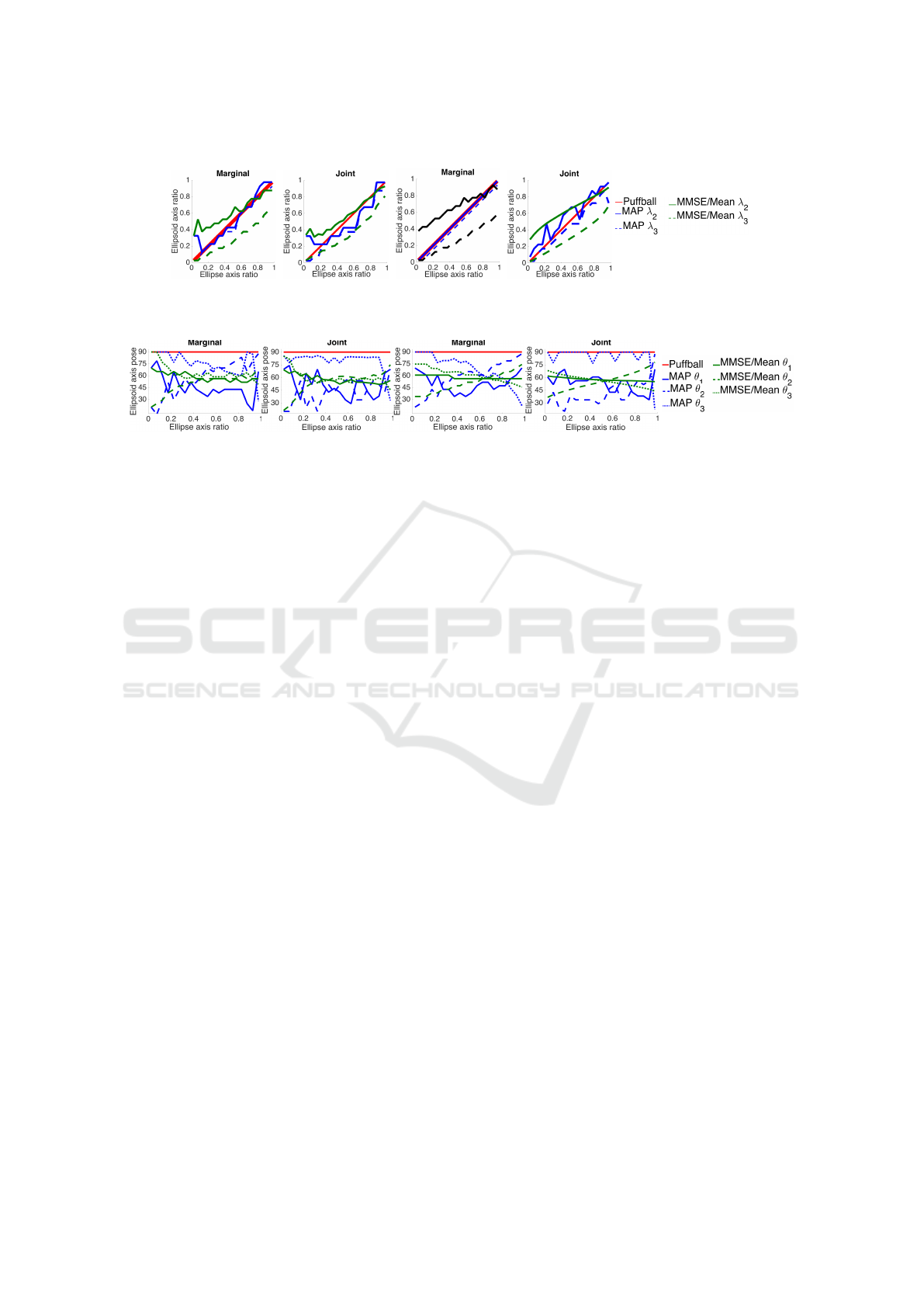
Fig. 7 shows the resulting estimators for shape and

Fig. 8 shows estimators for pose. Note that in the

Puffball solution the largest axis is always in the im-

age plane (θ

= 90 deg), and that λ

= λ

= m.

Consider ﬁrst the estimation of shape. Regardless

of prior and whether we are doing marginal or joint

estimation, the MAP solution follows Puffball fairly

closely. However, the MAP solution for shape does

deviate slightly from Puffball, and these deviations

are important (see below). A more profound diver-

gence from Puffball is seen in the MMSE and Mean

shape solutions, which in general return a losenge

rather than a cigar for all ellipses, with the two smaller

axes differing substantially in length.

Further insight can be gained by considering the

estimation of pose. Due to sampling error the MAP

solution is noisy, but it can be clearly seen that, un-

like Puffball, the major axis of the ellipsoid is slanted

away from the image plane by between 15 and 75 deg.

Note that, to be consistent with the observed ellipse,

this means that at least one of the smaller ellipsoid

axes must be slightly smaller than the puffball predic-

tion, a condition which can be veriﬁed from Fig. 7.

In the case of MMSE/Mean estimators, unlike

Puffball, the major axis of the ellipsoid does not tend

to lie in the image plane (θ

= 90 deg), but rather is

angled out of the image plane by roughly 30 deg on

VISAPP 2017 - International Conference on Computer Vision Theory and Applications

606

Empirical Prior Uniform Prior

Figure 7: Estimators for shape.

Empirical Prior Uniform Prior

Figure 8: Estimators for pose.

average (θ

= 60 deg). This is not too surprising, as

a uniform pose distribution (not conditioned on the

observation of ellipse) generates an average value for

,θ

and θ

of 1 radian (about 57 deg).

More interesting is the fact that the angle of the

major axis depends upon the ellipse shape: the ma-

jor axis of the ellipsoid is closer to the image plane

for more elongated ellipses. This is consistent with

the intuitions we expressed above. Since the empiri-

cal prior favours compact shapes, a highly elongated

ellipse is more likely to be generated by an ellip-

soid whose major axis is closer to the image plane.

Note, however, that we also see a variation, though

smaller, for the uniform prior. This may be due to

the generic view assumption: when conditioned on an

image measurement (in this case, an ellipse), a highly

elongated ellipsoid with major axis closer to the im-

age plane is favoured as it makes the observation more

stable with respect to angular perturbation, and thus

generates a higher conditional probability density.

There is even larger variation in the angle of the

second and third ellipsoid axes as a function of the

shape of the ellipse. For small ellipse ratios, the third

axis lies closer to the image plane, but for larger el-

lipse ratios the second axis lies closer to the image

plane. This makes sense because highly elongated

ellipses are more likely to be observed if the small-

est ellipsoid axis is close to the image plane, whereas

less elongated ellipses are more likely to be observed

if the second axis is close to the image plane.

6 QUANTITATIVE EVALUATION

We have seen that the MAP, MMSE and Puffball es-

timators make quite distinct predictions of ellipsoid

shape and pose from an observed ellipse. How does

this relate to the perception of more complex objects?

Suppose a more complex occluding contour is ob-

served. To obtain a rough estimate of 3D object shape

and pose, we could ﬁrst approximate this shape by an

ellipse and then use one of these estimators to infer an

ellipsoidal approximation of the 3D object, and/or its

pose. But which should we use?

To answer this question, we sampled 200 random

3D poses for each of the 61 shapes in our test dataset,

projected each to the image and used an ICP algo-

rithm to compute the best-ﬁtting ellipse to each ob-

served occluding contour. We used each of our meth-

ods to estimate an ellipsoidal approximation of the

original generating object from this observed ellipse.

We evaluated these ellipsoidal approximations by

computing the bidirectional mean-squared Euclidean

error between the estimated ellipsoid and the best-

ﬁtting ellipsoid for the ground truth object.

6.1 Shape Estimators

To evaluate the marginal shape estimators, each esti-

mated ellipsoid was scaled and rotated to minimize

the Euclidean distance from the ground truth ellip-

soid, and the resulting mean symmetric Euclidean dis-

tance was used as a measure of error. Fig. 9 reveals

that both MAP and MMSE shape estimators perform

better than Puffball, with MMSE performing best.

While the overlapping standard error bars in the

top panels of Fig. 9 might call into question the sta-

tistical signiﬁcance of these differences, these varia-

tions in error are highly correlated across estimators.

This correlated error can be factored out by consider-

ing the average reduction in error for each test shape

for the MAP and MMSE estimators relative to Puff-

Estimating Coarse 3D Shape and Pose from the Bounding Contour

607

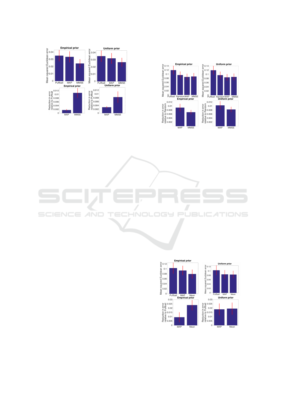
Figure 9: Top: Mean Euclidean error for marginal shape

estimation. Bottom: Reduction in error relative to Puffball

(larger is better).

ball (lower panels). From these plots it is easy to see

that the reduction in error is highly signiﬁcant for both

MAP and MMSE. Table 1 shows the percent reduc-

tion in mean error and also the percentage of shapes

for which error was lower for MAP and MMSE rel-

ative to Puffball. For MAP the improvement is rel-

atively modest (5-9%) but consistent: MAP is better

than Puffball for 75-97% of shapes. For MMSE the

mean improvement is more substantial (24-31%) but

less consistent: MMSE is better than Puffball for only

55-67% of shapes.

6.2 Pose Estimators

To evaluate the marginal pose estimators, we mea-

sured mean symmetric Euclidean error between

ground truth ellipsoid at the correct and estimated

poses. A problem emerges here: in our orthographic

projection framework, for each ellipsoid there are four

3D ’metamer’ poses that generate the same ellipse.

To handle this, when an estimator generates a pose,

we use an oracle to convert this to select from these

four metamers the pose that generates minimal error

relative to ground truth. Unfortunately, this puts Puff-

ball at a disadvantage, since it represents a degenerate

case where the four poses collapse to a single one. To

address this, we add as a baseline a random pose esti-

mator (Random), which selects a random pose, iden-

tiﬁes the four metamers and then selects the optimal

pose of these four using an oracle as described above.

As shown in Fig. 10, both MAP and MMSE pose

estimators perform better than both Puffball and Ran-

dom pose estimators. Since the Random estimator

performs better than Puffball, we evaluate the per-

formance of MAP and MMSE estimators relative to

the latter (Fig. 10, bottom panels and Table 2.) Both

MAP and MMSE generate signiﬁcantly more accu-

rate pose estimates. While MAP generates slightly

greater mean improvement, improvements are more

consistent across objects for MMSE.

Figure 10: Top: Mean Euclidean error for marginal pose

estimation. Bottom: Reduction in error relative to the Ran-

dom pose estimator (larger is better).

6.3 Joint Conﬁguration Experiments

For the joint estimators, symmetric Euclidean error of

each estimated ellipsoid relative to the ground truth

ellipsoid is computed, with no scaling or rotation.

Again, an oracle is used to select the pose that yields

lowest error, and this does put Puffball at a disadvan-

tage. Unfortunately it is difﬁcult to correct for this

for joint shape-pose estimation, as selecting a random

pose but using the Puffball shape would no longer

be consistent with the observed ellipse. We there-

fore present results without correction, noting that the

marginal shape and pose results presented above con-

ﬁrm that our MAP and MMSE estimators outperform

Puffball for both of these dimensions individually.

Fig. 11 shows that for the empirical prior, the

Mean estimator is best, while for the uniform prior,

MAP and Mean are comparable. Table 3 shows that

Figure 11: Mean Euclidean error for joint estimation. Bot-

tom: Reduction in error relative to Puffball (larger is better).

the Mean estimator generates a greater average im-

VISAPP 2017 - International Conference on Computer Vision Theory and Applications

608

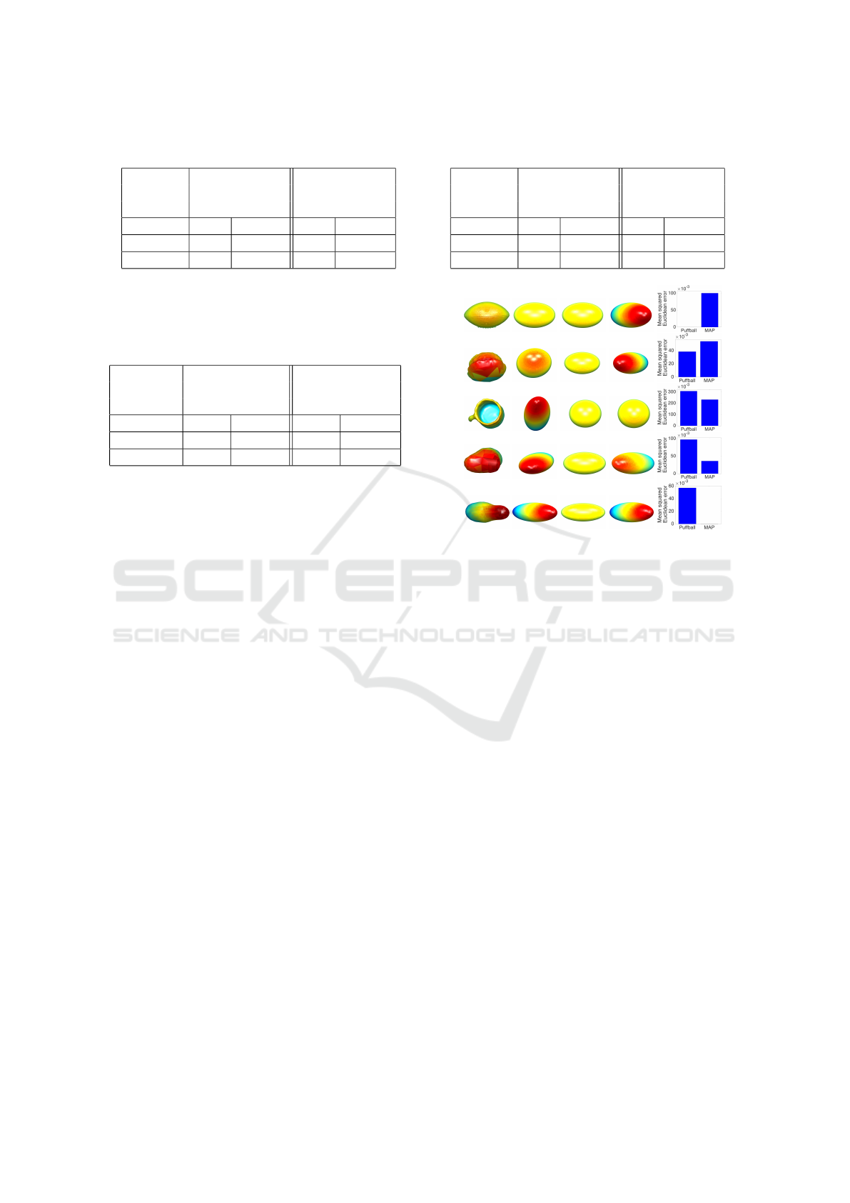
Table 1: Performance of MAP and MMSE shape estimators

relative to Puffball.

Prior Mean reduction % of objects for

in error which error is

reduced

MAP MMSE MAP MMSE

Empirical 5% 31% 75% 67%

Uniform 9% 24% 97% 55%

Table 2: Performance of MAP and MMSE pose estimators

relative to the Random pose estimator.

Prior Mean reduction % of objects for

in error which error is

reduced

MAP MMSE MAP MMSE

Empirical 10% 7% 87% 98%

Uniform 11% 9% 92% 98%

provement for the Empirical prior, but the MAP esti-

mator is more reliable for the uniform prior.

Table 3: Performance of MAP and MMSE joint shape-pose

estimators relative to Puffball.

Prior Mean reduction % of objects for

in error which error is

reduced

MAP Mean MAP Mean

Empirical 9% 23% 70% 70%

Uniform 18% 19% 87% 67%

7 QUALITATIVE EVALUATION

To get a qualitative sense of the performance of our

joint shape-pose estimators, Figs. 12-13 show repre-

sentative results for speciﬁc shapes in our test dataset,

using MAP and Mean estimators based on our em-

pirical prior. To generate Fig. 12, we ﬁrst sorted the

test cases by percent reduction in mean error for MAP

over Puffball, and then show 0th, 25th, 50th, 75th and

100th percentile examples. The ﬁrst (0th percentile)

case is the shape for which MAP performs worst rel-

ative to Puffball. The last (100th percentile) case is

the shape for which MAP has the largest error reduc-

tion relative to Puffball. The third (50th percentile)

case is the median (representative) example. Simi-

larly, Fig. 13 compares the Mean solution to Puffball.

In these qualitative comparisons, we note the el-

liptical projections of the estimated ellipsoids do not

exactly match, and are sometimes quite different from

the elliptical projections of the ground truth ellip-

soids. This is primarily because the estimated ellip-

soids are conditioned on an ellipse ﬁtted in the image

plane to the projected object, and in general this el-

lipse is different from the elliptical projection of the

ground truth ellipsoid.

In addition, for a given shape there are small vari-

ations between the elliptical projections of the esti-

mated ellipsoids. This is due to the ﬁnite sampling of

shape and pose space.

Despite these limitations, the qualitative results

are interesting. It is probably most instructive to con-

sider the median results (third row) as these are repre-

(a)

Object

(b)

Ground

truth

ball

(d)

MAP

(e) Error

Figure 12: Examples of joint shape-pose estimation on test

set objects. Objects were ranked according to the percent

reduction in mean error for MAP over Puffball estimator.

From top to bottom: 0, 25, 50, 75, and 100 percentile ob-

jects.

sentative. In both cases of Fig. 12 and 13, the statisti-

cal estimators have smaller errors relative to Puffball.

Interestingly, in Fig. 13, the Mean estimator is able to

capture the greater elongation and out-of-plane rota-

tion of the object that Puffball is unable to capture.

8 CONCLUSIONS AND FUTURE

WORK

In this paper we set out to understand whether coarse

3D shape information could be extracted from object

silhouettes even under orthographic projection. In

particular, we conjectured that the tendency for ob-

jects to be compact and the generic view assumption

should together bias the rough shape and pose when

conditioned on the silhouette. Our experimental re-

sults conﬁrm this hypothesis.

One limitation of this study is the use of an

oracle to distinguish between four metamer poses

in marginal pose and joint shape-pose estimations.

Estimating Coarse 3D Shape and Pose from the Bounding Contour

609

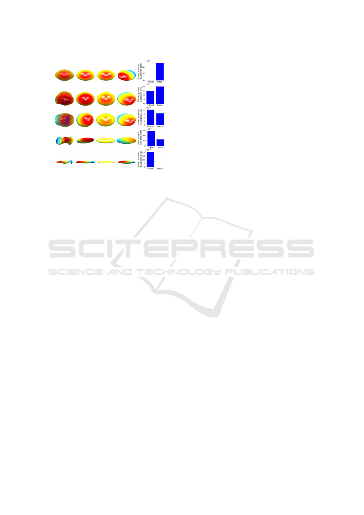
(a)

Object

(b)

Ground

truth

ball

(d)

Mean

(e) Error

Figure 13: Examples of joint shape-pose estimation on test

set objects. Objects were ranked according to the percent

reduction in mean error for Mean over Puffball estimator.

From top to bottom: 0, 25, 50, 75, and 100 percentile ob-

jects.

Since this limitation is a direct consequence of or-

thographic projection, an obvious next step is to use

perspective projection, which will disambiguate these

metamers and allow us to do a fairer comparison.

Even with statistically optimal estimators, given

only elliptical approximations, shape and pose esti-

mation is quite unreliable. The value of this work thus

lies not in immediate application, but rather in the in-

tegration of these estimators with additional boundary

shape cues as well as weak surface cues (e.g., shad-

ing, texture) that are usually present in the image but

often insufﬁcient to fully constrain 3D reconstruction.

REFERENCES

Barron, J. T. and Malik, J. (2015). Shape, illumination, and

reﬂectance from shading. IEEE Transactions on Pat-

tern Analysis and Machine Intelligence, 37(8):1670–

1687.

Besl, P. J. and McKay, H. D. (1992). A method for regis-

tration of 3-d shapes. IEEE Transactions on Pattern

Analysis and Machine Intelligence, 14(2):239–256.

Blum, H. (1973). Biological shape and visual science (Part

I). J. Theor. Biol., 38:205–287.

C¸ alli, B., Walsman, A., Singh, A., Srinivasa, S., Abbeel, P.,

and Dollar, A. M. (2015). Benchmarking in manip-

ulation research: The YCB object and model set and

benchmarking protocols. ArXiv e-prints.

Cole, F., Isola, P., Freeman, W., Durand, F., and Adelson,

E. (2012). Shapecollage: Occlusion-aware, example-

based shape interpretation. In Fitzgibbon, A., Lazeb-

nik, S., Perona, P., Sato, Y., and Schmid, C., edi-

tors, Computer Vision ECCV 2012, volume 7574 of

Lecture Notes in Computer Science, pages 665–678.

Springer Berlin Heidelberg.

Elder, J. H. (2014). Bridging the dimensional gap: Per-

ceptual organization of contour into two-dimensional

shape. In Wagemans, J., editor, Oxford Handbook of

Perceptual Organization, Oxford, UK. Oxford Uni-

versity Press.

Freeman, W. T. (1994). The generic viewpoint assump-

tion in a framework for visual perception. Nature,

368(6471):542–545.

Igarashi, T., Matsuoka, S., and Tanaka, H. (1999). Teddy:

a sketching interface for 3D freeform design. In Pro-

ceedings of the 26th annual conference on computer

graphics and interactive techniques, SIGGRAPH

’99, pages 409–416, New York, NY, USA. ACM

Press/Addison-Wesley Publishing Co.

Karsch, K., Liao, Z., Rock, J., Barron, J. T., and Hoiem,

D. (2013). Boundary Cues for 3D Object Shape Re-

covery. In Computer Vision and Pattern Recogni-

tion (CVPR), 2013 IEEE Conference on, pages 2163–

2170.

Koenderink, J. (1984). What does the occluding contour tell

us about solid shape? Perception, 13(321-330).

Oswald, M., Toppe, E., Kolev, K., and Cremers, D. (2009).

Non-parametric single view reconstruction of curved

objects using convex optimization. In Denzler, J.,

Notni, G., and S

ue, H., editors, Pattern Recognition,

volume 5748 of Lecture Notes in Computer Science,

pages 171–180. Springer Berlin Heidelberg.

Prasad, M., Zisserman, A., and Fitzgibbon, A. W. (2006).

Single view reconstruction of curved surfaces. In

Computer Vision and Pattern Recognition, 2006 IEEE

Computer Society Conference on, volume 2, pages

1345–1354.

Singh, A., Sha, J., Narayan, K. S., Achim, T., and Abbeel, P.

(2014). Bigbird: A large-scale 3D database of object

instances. In 2014 IEEE International Conference on

Robotics and Automation (ICRA), pages 509–516.

Todd, J. (2004). The visual perception of 3D shape. Trends

in Cognitive Sciences, 8(3):115–121.

Todd, J. T. and Reichel, F. D. (1989). Ordinal structure

in the visual perception and cognition of smoothly

curved surfaces. Psychological Review, 96(4):643–

657.

Toppe, E., Oswald, M. R., Cremers, D., and Rother, C.

(2011). Image-based 3D Modeling via Cheeger Sets.

In Proceedings of the 10th Asian Conference on Com-

puter Vision - Volume Part I, ACCV’10, pages 53–64,

Berlin, Heidelberg. Springer-Verlag.

Tse, P. (2002). A contour propagation approach to surface

ﬁlling-in and volume formation. Psychological Re-

view, 109(1):91–115.

Twarog, N. R., Tappen, M. F., and Adelson, E. H. (2012).

Playing with Puffball: Simple scale-invariant inﬂa-

tion for use in vision and graphics. In Proceedings

of the ACM Symposium on Applied Perception, SAP

’12, pages 47–54, New York, NY, USA. ACM.

VISAPP 2017 - International Conference on Computer Vision Theory and Applications

610