
On the Impact of using Mixed Integer Programming Techniques on
Real-world Offshore Wind Parks
Martina Fischetti
1,2
and David Pisinger
2
1
Vattenfall BA Wind, Jupitervej 6, 6000 Kolding, Denmark
2
Technical University of Denmark, Operations Research, DTU Management,
Produktionstorvet, 424 DK-2800 Kgs. Lyngby, Denmark
Keywords:
Optimization, Mixed Integer Linear Programming, Wind Energy, Routing, Offshore Cables, Green Energy.
Abstract:
Wind power is a leading technology in the transition to sustainable energy. Being a new and still more compet-
itive field, it is of major interest to investigate new techniques to solve the design challenges involved. In this
paper, we consider optimization of the inter-array cable routing for offshore wind farms, taking power losses
into account. Since energy losses in a cable depend on the load (i.e. wind), cable losses are estimated by con-
sidering a possibly large number wind scenarios. In order to deal with different wind scenarios efficiently we
used a precomputing strategy. The resulting optimization problem considers two objectives: minimizing im-
mediate costs (CAPEX) and minimizing costs due to power losses. This makes it possible to perform various
what-if analyses to evaluate the impact of different preferences to CAPEX versus reduction of power losses.
Thanks to the close collaboration with a leading energy company, we have been able to report results on a
set of real-world instances, based on six existing wind parks, studying the economical impact of considering
power losses in the cable routing design phase.
1 INTRODUCTION
With a total global capacity of more than 400 GW
by the end of 2015, wind power is a leading technol-
ogy in the transition away from fossil fuels. Having
a yearly market growth of 15-20%, it is however nec-
essary to face new challenges on a market that is al-
ways more competitive. According to [Gonzlez et al.,
2014] the expenses for electrical infrastructure of a
offshore wind farm account for 15-30% of the over-
all initial costs. Therefore, high-level optimization in
this area is a key factor. In this work we focus on the
cable routing between offshore wind turbines (the so
called inter-array optimization).
The power production of offshore turbines is col-
lected through one or more substations and then con-
veyed to the coast. The cabling will therefore con-
stitute a tree of cables from each substation to the
connected turbines. Different cables with different
costs, capacities and resistances are available on the
market and the task is therefore not only to connect
the turbines in the cheapest possible way, but also to
choose appropriate dimensions of the cables to mini-
mize losses.
Thanks to the collaboration with a leading energy
company it has been possible to build a detailed model
including nearly all the constraints arising in practical
applications, and to evaluate the savings of optimized
layouts on real cases. The resulting optimization tool
has been validated by company experts, and is now
routinely used by the planners.
Wind park cable routing optimization has ob-
tained considerable attention in the last years. Due to
the large number of constraints and the intrinsic com-
plexity of the problem, many studies (i.e. [Dutta and
Overbye, 2011, Gonzlez-Longatt and Wall, 2012, Li
et al., 2008, Zhao et al., 2009]) preferred to use ad-
hoc heuristics. Only a few papers used Mixed Inte-
ger Linear Programming (MILP), notably [Bauer and
Lysgaard, 2015, Fagerfjall, 2010, Dutta, 2012, Berzan
et al., 2011,Hertz et al., 2012,Cerveira et al., 2016,Pil-
lai et al., 2015]. A MILP approach boosted with
heuristics (a so-called mat-heuristic approach) to deal
with large-scale wind parks in an acceptable time
has been recently proposed in [Fischetti and Pisinger,
2016]. The present work is based on [Fischetti and
Pisinger, 2016] but focuses more on real applications
of the optimization model and on its economical im-
pact. Several variants of the problem have been pro-
posed in the literature. To the best of our knowledge
108
Fischetti M. and Pisinger D.
On the Impact of using Mixed Integer Programming Techniques on Real-world Offshore Wind Parks.
DOI: 10.5220/0006190701080118
In Proceedings of the 6th International Conference on Operations Research and Enterprise Systems (ICORES 2017), pages 108-118
ISBN: 978-989-758-218-9
Copyright
c
2017 by SCITEPRESS – Science and Technology Publications, Lda. All rights reserved

only [Cerveira et al., 2016] has considered power loss
in cables. However, [Cerveira et al., 2016] does not
take into account variable cable loads due to fluc-
tuating wind. [Bauer and Lysgaard, 2015] proposes
an Open Vehicle Routing approach for this problem
adding the planarity constraints on the fly. In this
Open Vehicle Routing version of the problem, only
one cable can enter a turbine, even if this is often
not the case in the reality. In [Bauer and Lysgaard,
2015], the possibility of branching cables in the tur-
bines (as we are doing), is mentioned as a future work.
However, the substation limits, that could be a major
constraint in practical applications, are not considered
in [Bauer and Lysgaard, 2015]. Different approaches
for the cable network design are provided in [Berzan
et al., 2011]. The suggested approach is a divide-and-
conquer heuristic based on the idea of dividing the
big circuit problem into smaller circuit problems. The
proposed MILP model cannot deal with more than 11
turbines. In [Hertz et al., 2012] the cable layout prob-
lem for onshore cases is studied. The onshore cable
problem is similar to the offshore one with the fol-
lowing differences. First of all, the cable can be of
two types: underground cables (connecting turbines
to other turbines or to the above-ground level), and
above-ground cables. In the first case, the cables need
to be dug in the ground. Due to the fact that parallel
lines can use the same dug hole, parallel structures are
preferred (until a fixed number). The above-ground
level cables need to follow existing roads. Such con-
straints do not exist in the offshore case.
The main contribution of this paper is to anal-
yse how the inter-array cable routing of real-world
wind farms can be improved by using modern opti-
mization techniques. A particularly challenging as-
pect in the cable routing design, is to understand if
one could limit power losses by optimizing cable rout-
ing. As a general rule, cables with less resistance are
also more expensive, therefore we would like here to
make a proper trade-off between investments and ca-
ble losses. We formulate the optimization problem
with immediate costs (CAPEX) and losses-related
costs as two separate goals. The two objectives can be
merged into a single objective by proper weighing of
the two parts. The weighing factor can be considered
fixed or can vary: this makes it possible to perform
various what-if analyses to evaluate the impact of dif-
ferent preferences (i.e. of different weighing factors).
The latter approach is important in cases where a pos-
itive pay-back is demanded within a short time hori-
zon, or where liquidity problems hinder choosing the
best long-term solution. We report a study of both
approaches on a set of real-world instances.
In order to perform the above analysis, we devel-
oped a MIP approach to optimize the routing. In the
computation of power losses, it is shown that wind
scenarios can be handled efficiently as part of data
preprocessing, resulting in a MIP model of tractable
size. Tests on a library of real-life instances proved
that substantial savings can be achieved.
The rest of the paper is organized as follows: Sec-
tion 2 describes our MILP model, first presenting a
basic model and then improving and extending the
formulation. In particular, we show how to model
power losses, and propose a precomputing strategy
that is able to handle this non-linearity efficiently, thus
avoiding sophisticated quadratic models that would
make our approach impractical. Section 3 compares
our optimized solutions with an existing cable layout
for a real wind farm (Horns Rev 1), showing that mil-
lions of euro can be saved. Section 4 is dedicated to
various what-if analyses. Subsection 4.1 describes the
real-world wind farms that we considered in our tests
while Subsection 4.2 shows the results of our opti-
mization on a testbed of real-world cases, reporting
the impact of considering power losses for all the in-
stances. Subsection 4.3 is dedicated to the Pareto opti-
mality study. Some conclusions are finally addressed
in Section 5.
2 MATHEMATICAL MODEL FOR
CABLE ROUTING
OPTIMIZATION
2.1 Basic Model
In the present paper we assume that the location of the
turbines has already been defined. We wish to find an
optimal cable connection between all turbines and the
given substation(s), minimizing the total cable costs.
The optimization problem considers that:
• the energy flow leaving a turbine must be sup-
ported by a single cable;
• the maximum energy flow (when all the turbines
produce their maximum) in each connection can-
not exceed the capacity of the installed cable;
• different cables, with different capacities, costs
and impedances, can be installed;
• cable crossing should be avoided;
• a given maximum number of cables can be con-
nected to each substation;
• cable losses (dependent on the cable type, the ca-
ble length and the current flow through the cable)
must be considered in the optimization.
On the Impact of using Mixed Integer Programming Techniques on Real-world Offshore Wind Parks
109

We will first model the problem without cable
losses and then discuss in Subsection 2.2 how to effi-
ciently express these constraints. We model turbine
positions as nodes of a complete and loop-free di-
rected graph G = (V, A) and all possible connections
between them as directed arcs. Some nodes corre-
spond to the substations that are considered as the
roots of the trees, being the only nodes that collect
energy. Let P
h
be the power production at node h. We
distinguish between two different types of node:
h ∈
V
T
if the h-th node correspond to a turbine
V
0
if the h-th node correspond to a substation
Let T denote the set of different cable types that
can be used. Each cable type t has a given capacity k
t
and unit cost u
t
, representing the cost per meter of the
cable (CAPEX). Arc costs can therefore be defined as
c
t
i, j
= dist(i, j)u
t
for each arc (i, j) and for each type
t ∈ T , where dist(i, j) is the distance between turbine
i and turbine j. In our model we use the continuous
variables f
i, j
≥ 0 for the maximum flow on arc (i, j).
The binary variables x
t
i, j
define cable connections as
x
t
i, j
=
(
1 if arc (i, j) with cable type t is selected
0 otherwise
Finally, variables y
i, j
indicate whether turbines
i and j are connected (with any type of cable).
Note that variables y
i, j
are related to variables x
t
i, j
as
∑
t∈T
x
t
i, j
= y
i, j
. The overall model becomes:
min
∑
i, j∈V
∑
t∈T
c
t
i, j
x
t
i, j
(1)
s.t.
∑
t∈T
x
t
i, j
= y
i, j
i, j ∈ V : j 6= i (2)
∑
i:i6=h
( f
h,i
− f
i,h
) = P
h
h ∈ V
T
(3)
∑
t∈T
k
t
x
t
i, j
≥ f
i, j
i, j ∈ V : j 6= i, (4)
∑
j: j6=h
y
h, j
= 1 h ∈ V
T
(5)
∑
j: j6=h
y
h, j
= 0 h ∈ V
0
(6)
∑
i6=h
y
i,h
≤ C h ∈ V
0
(7)
x
t
i, j
∈ {0, 1} i, j ∈ V, t ∈ T (8)
y
i, j
∈ {0, 1} i, j ∈ V (9)
f
i, j
≥ 0 i, j ∈ V, j 6= i (10)
The objective function (1) minimizes the total cable
layout cost. Constraints (2) impose that only one type
of cable can be selected for each built arc, and defines
the y
i, j
variables. Constraints (3) are flow conserva-
tion constraints: the energy (flow) exiting each node h
is equal to the flow entering h plus the power produc-
tion of that node (except if the node is a substation).
Constraints (4) ensure that the flow does not exceed
the capacity of the installed cable, while constraints
(5) and (6) impose that only one cable can exit a tur-
bine and none can exit the substations (tree structure
with root in the substations). Finally, constraints (7)
impose the maximum number of cables (C) that can
enter each substation.
In order to model no-crossing constraints we need
a constraint for each pair of crossings arcs, i.e. a
huge number of constraints. We have, therefore, de-
cided to generate them on the fly, as also suggested
in [Bauer and Lysgaard, 2015]. In other words, the
optimizer considers model (1) - (10) and adds the
following new constraints whenever two established
connections (i, j) and (h, k) cross
y
i, j
+ y
j,i
+ y
h,k
+ y
k,h
≤ 1. (11)
The reader is referred to [Fischetti and Pisinger, 2016]
for stronger versions of those constraints. Using
this approach, the number of non-crossing constraints
actually added to the model decreases dramatically,
making the model faster to solve. As presented,
the model is able to deal with small size instances
only. In order to produce high quality solutions in
an acceptable amount of time also for big instances
a “matheuristic” framework (as the one proposed in
[Fischetti and Pisinger, 2016]) should be used on top
of this basic model.
2.2 Cable Losses
In this section we propose an extension of the previ-
ous model taking cable losses into account. Let us
consider a generic cable (i, j) of type t, supporting a
current g
t
i, j
. Power losses increase with the square of
the current, according to the formula:
3R
t
· dist(i, j)(g
t
i, j
)
2
(12)
where R
t
is the electrical resistance of the 3-phase
cable of type t, in Ω/m. The current g
t
i, j
obviously
depends on the considered wind scenario. As a con-
sequence, dealing with equation (12) directly in the
model, would imply dealing with non-linearities over
multiple scenarios. Nevertheless, (12) can be sim-
plified if we assume that all the turbines in the park
have the same power production under the same wind
scenario. This is a fair assumptions since typical
parks are constructed by using only one turbine model
and wake effect is not usually considered in electrical
studies. Under this assumption, the current I
s
passing
through a generic cable (i, j) of type t under scenario
s, can be expressed as a function of the number f of
turbines supported by the cable as:
PLoss
t, f ,s
= ( f I
s
)
2
R
t
dist(i, j). (13)
The value f = 1, ...F is limited by the capacity of the
cables. By introducing the dependency on f in our
ICORES 2017 - 6th International Conference on Operations Research and Enterprise Systems
110

main binary variables (now x
t, f
i, j
) we can re-write our
two objectives as:
min
∑
i, j∈V
∑
t∈T
∑
f ∈F
∑
s∈S
π
s
PLoss
t, f ,s
x
t, f
i, j
(14)
and
min
∑
i, j∈V
∑
t∈T
∑
f ∈F
c
t
i, j
x
t, f
i, j
(15)
where π
s
is the probability of scenario s. As we have
discussed earlier, minimizing losses can imply an in-
crease of the CAPEX cost, therefore the two objective
must be properly balanced. In some cases (e.g., when
there is no limit on the CAPEX) they can be merged,
by using a converting factor for the loss-related term:
this is the estimated cost for each MW of production
lost over the wind farm lifetime (Net Present Value).
This value (denoted as K) is an input value, that the
designer can set to the desired project-specific value.
The merged objective function, now expressed in e,
is then:
min
∑
i, j∈V
∑
t∈T
∑
f ∈F
c
t
i, j
x
t, f
i, j
+K
∑
i, j∈V
∑
t∈T
∑
f ∈F
∑
s∈S
π
s
PLoss
t, f ,s
x
t, f
i, j
(16)
We notice that (16) can be rewritten as:
min
∑
i, j∈V
∑
t∈T
∑
f ∈F
u
t
dist(i, j)x
t, f
i, j
+K
∑
i, j∈V
∑
t∈T
∑
f ∈F
∑
s∈S
3π
s
( f I
s
)
2
R
t
dist(i, j)x
t, f
i, j
=
min
∑
i, j∈V
∑
t∈T
∑
f ∈F
(u
t
+ K
∑
s∈S
3π
s
( f I
s
)
2
R
t
)dist(i, j)x
t, f
i, j
(17)
The non-linear expressions in the objective func-
tion (17) can actually be handled implicitly in a
pre-processing phase, without changing the original
model (1)-(10) at all, according to the following idea.
We consider the basic model (1)–(10) without cable
losses on a modified instance where each cable type
is replaced by a series of “subcables” with discretized
capacity and modified cable cost taking both CAPEX
and revenue losses due to cable losses into account.
Nearly all wind farms are designed for only one
turbine type, hence the maximum power production
P
h
of each turbine can be assumed to be 1, meaning
that we can express the cable capacity as the maxi-
mum number of turbines supported. Consider a cer-
tain cable type t that can support up to k
t
turbines. We
replace it by k
t
“subcable” types of capacity f = 1, 2,
..., k
t
whose unit cost is computed by adding both ca-
ble/installation unit costs (u
t
) and loss costs (denoted
as loss
t, f
) considering the current produced by exactly
f turbines. Note that such unit costs increase with f ,
so the optimal solution will always select the subca-
ble type f supporting exactly the number of turbines
connected, hence the approach is correct.
The above approach allows us to easily consider
multiple wind scenarios without affecting the model
size. This is obtained by precomputing the subcable
costs by just considering a weighted average of the
loss cost under different wind scenarios (and hence
different current productions). To be more specific, if
we look again at formula (17), we can now precom-
pute the value
loss
t, f
= K
∑
s∈S
3π
s
( f I
s
)
2
R
t
(18)
where π
s
is the probability of scenario s and I
s
is the
current produced by a single turbine under wind sce-
nario s, assuming negligible wake effect, i.e., all tur-
bines are producing the same amount of energy under
a given wind scenario s. We refer to the next subsec-
tion for a more detailed example of how cable costs
are pre-processed when considering losses. As said,
K is a factor to estimate the value (in e) of the MW
loss, and can be computed as K = K
euro
· 8760 where
K
euro
is the NPV for a MW/h production over the park
lifetime, and 8760 is the number of hours in a year.
Notice that K
euro
acts as a weighting factor between
the two objectives: minimize CAPEX costs versus
minimize losses.
2.3 Loss Pre-computation
In this section we elaborate on our pre-computing
strategy proposed in the previous session, using a con-
crete example from the real wind park Horns Rev 1.
The park consists of 80 2MW turbines and is located
about 15 km from the Danish shore. This park will be
used as one of our test cases both in Section 3 and 4.
Fixed the turbine layout, one could consider dif-
ferent sets of cables to be used. Different sets can
differ in cable cross section or in voltage (33kV or
66kV generally), which reflects in different capacities
and resistances. The set of most adequate cables is se-
lected by the electrical specialists in the company. Of
course, different cables can lead to different solutions,
as we will see in Section 4.
We will now focus on one cable set only, in order
to better illustrate how different wind scenarios are
handled in the pre-processing phase. Changing the
cable data, the process is analogous.
Let us suppose that we are given a set of two ca-
bles: the cheapest one can support ten 2MW turbines
and the most expensive fourteen turbines. This set
of cables will be indicated as cb05 in Section 4. We
are provided with the following table, that reports the
characteristics of the two cable types.
If we want to optimize on CAPEX costs only, we
just need to input to the model the capacity of each
On the Impact of using Mixed Integer Programming Techniques on Real-world Offshore Wind Parks
111

Table 1: Cable information for cb05.
n. of resistance price install. price
cables type 2MW turb. [Ohm/km] [e/m] [e/m]
cb05
1 10 0.13 180 260
2 14 0.04 360 260
cable type and its overall cost (cable price plus instal-
lation cost). In this case, for example, this would be:
• type 1: supports up to 10 turbines with a unit cost
of 440 e/m
• type 2: supports up to 14 turbines with a unit cost
of 620 e/m
Table 2 shows how the model will compute the unit
price (CAPEX only) depending on the number of tur-
bines connected.
Table 2: CAPEX costs for cb05, depending on the number
of turbines connected.
n. of 2MW price
cable type turb. supported [e/m]
1
1 440
2 440
3 440
4 440
5 440
6 440
7 440
8 440
9 440
10 440
2
11 620
12 620
13 620
14 620
Notice that, considering CAPEX costs only, the
cost to use one type of cable is independent of how
many turbines it is connected to (up to the capacity
limit).
Let us now consider the losses in our optimization
using the strategy of Subsection 2.2. As we discussed
earlier, the power loss in a cable depends on the cur-
rent passing through it. Since only a discrete number
of turbines can be connected to each cable path, we
can express the current as a function of the number f
of turbines connected (as shown equation (18)) with-
out any loss of precision in the result.
Still referring to equation (18), the losses depend
also on the wind statistics in the site. We can define a
wind scenario (s) as a wind speed and its probability
to occur (π
s
). At a given wind speed, a given turbine
will produce a specific current (I
s
).
Wind scenarios can be defined in different ways.
In this paper we used both real measurements and sce-
narios derived from Weibull distributions for the spe-
cific sites. For the Horns Rev 1 case we are consid-
ering, we had real measurements from the site, i.e., a
wind speed sample each 10 minutes for 10 years. We
grouped all these samples in wind-speed bins of 1m/s,
obtaining 25 wind scenarios (from 1 m/s to 25 m/s).
The probability of each scenario was obtained looking
at the frequency of the specific wind speed over all the
samples. In our tests we decided to bin our data ev-
ery 1 m/s, following the practice in electrical losses
computations. However this should not be considered
a limit: since the wind scenarios are handled in the
pre-processing phase, the number of scenarios does
not affect the size of the final optimization model.
Having computed I
s
and π
s
according to the sce-
nario definition, power losses can now be calculated.
Parameter K
euro
= 690 e/MWh was computed by the
company experts for a wind park lifetime of 25 years,
while resistance R
t
is defined according to Table 1.
Using equation (18), power loss costs loss
t, f
can be
now precomputed. As shown in (17), the cost con-
sidered in the objective for each cable connection will
need to include the CAPEX costs (u
t
) and the contri-
bution from losses (loss
t, f
). Therefore the final imput
to the optimization tool for Horns Rev 1 with cb05,
will be as shown in Table 3.
Table 3: Precomputed cable prices for cable cb05 (including
installation costs) precomputed considering fixed costs and
power losses for Horns Rev 1.
n. of 2MW price
cable type turb. supported [e/m]
1
1 441.16
2 442.71
3 445.27
4 448.87
5 453.50
6 459.15
7 465.83
8 473.54
9 482.28
10 492.04
2
11 639.77
12 643.41
13 647.36
14 651.63
A comparison between Tables 2 and 3 shows the
impact of considering losses on cable prices. While
from a installation perspective the cost for each cable
type is fixed, it now varies depending on how many
turbines are connected. As we will see, this can have
an impact on the optimal cable routing.
ICORES 2017 - 6th International Conference on Operations Research and Enterprise Systems
112
3 COMPARISON WITH AN
EXISTING LAYOUT
We report in this section a comparison between our
optimized solutions (considering and not considering
losses) and the existing cable routing for Horns Rev 1,
a real-world offshore park located in Denmark. Fig-
ure 1 shows the actual design for Horns Rev 1 (from
[Kristoffersen and Christiansen, 2003]).
Figure 1: Existing cable routing for Horns Rev 1.
Three different types of cables are used: the
thinnest cable supports one turbine only, the medium
supports 8 turbines, and the thickest 16. We estimated
the costs and resistances of these cables based on the
cable cross section. The estimated prices are 85 e/m,
125 e/m and 240 e/m, respectively, plus an estimated
260e/m of installation costs (independent of the ca-
ble type). We ran our CAPEX optimization with the
above prices obtaining the layout in Figure 2. The
optimized layout is significantly different from the ex-
isting one. Looking at immediate costs, the optimized
layout is over 1.5 Me less expensive. As already said,
this layout is optimized only on immediate costs, nev-
ertheless if we estimate its value in 25 years (consid-
ering losses) this layout is still more profitable than
the existing one: considering both CAPEX and losses
the optimized layout is 1.6 Me more profitable than
the existing one (Net Present Value) .
By optimizing cable losses, one can further in-
crease the value in the long term. Figure 3 shows
the optimized solution considering losses (thus opti-
mizing the value of the cable route in its lifetime).
Compared with the existing layout (Figure 1), this
new layout is about 1.7 Me (NPV) more profitable
in 25years, and still around 1.5 Me cheaper at con-
Figure 2: Optimized layout for Horns Rev 1 (CAPEX costs
only): this layout results more than 1.5M e more profitable
than the existing one.
Figure 3: Optimized layout for Horns Rev 1 (considering
losses): in the wind park lifetime this layout is estimated to
be more than 1.7Me more profitable than the existing one.
struction time.
Table 4 summarizes the savings of the two opti-
mized layouts compared with the existing one, both
from an immediate cost perspective and from a long-
term perspective: values are expressed in Ke.
The test shows that millions of euros can be saved
using our optimization methods on real parks. In the
next section we want to focus on the other great ad-
vantage of using automatic optimization tools: the
possibility of performing a number of what-if anal-
yses. To the best of our knowledge, this is the first de-
On the Impact of using Mixed Integer Programming Techniques on Real-world Offshore Wind Parks
113

Table 4: Savings of optimized solutions compared with the
existing cable routing for Horns Rev 1.
Savings [Ke]
opt mode immediate in 25years
CAPEX 1544 1605
lifetime 1511 1687
tailed study on the impact of different design choices
on the cable routing itself and on its impact on imme-
diate costs (CAPEX) and long term costs.
4 WHAT-IF ANALYSIS
We performed a number of what-if analyses on dif-
ferent real-world wind farms. In particular we were
interest in understanding the impact of considering
power losses in the design phase. We will first com-
pare solutions optimized only for CAPEX costs, with
solutions optimized looking at the whole lifetime of
the park. We will then study the usage of differ-
ent types of cable (with different resistances) in both
cases, and the long-term savings compared with the
possible higher investments costs. We will also per-
form a multi-criteria analysis where the user can bal-
ance between initial costs and long-term savings: this
could be of interest, for example, when the company
requests that the higher investment must be paid off
in a limited number of years.
4.1 Test Instances
We tested our model on the real-world instances pro-
posed in [Fischetti and Pisinger, 2016]. They consider
five different real wind farms in operation in United
Kingdom and Denmark, and one new wind farm un-
der construction. These parks are Horns Rev 1, Ken-
tish Flats, Ormonde, Dan Tysk, Thanet and Horns Rev
3.
This dataset includes old and new parks, with dif-
ferent power ratings and different number of turbines
installed, and therefore represents a good benchmark
for our tests. Each park has one substation with its
own maximum number of connections (C).
In details:
• Horns Rev 1 has 80 turbines Vestas 80-2MW and
C = 10
• Kentish Flats has 30 turbines Vestas 90-3MW. It
is a near-shore wind farm, so it is connected to
the onshore electrical grid without any offshore
substation. Nevertheless, only one export cable is
connected to the shore, therefore the starting point
of the export cable is treated as a substation. We
set C = ∞ as there is no physical substation limi-
tation in this case.
• Ormonde has 30 Senvion 5MW and C = 4
• DanTysk has 80 Siemens 3.6MW and C = 10
• Thanet has 100 Vestas 90-3MW and C = 10
• Horns Rev 3 has 50 Vestas 164-8MW and C = 12
The dataset also includes different sets of cables,
indicated as cb01, cb02, cb03, cb04 and cb05.
The cost of the cables considering power losses
has been precomputed following the strategy pro-
posed in Subsection 2.2. We computed the cable-loss
prices using real measured data (for Horns Rev 1 and
3, Ormonde and DanTysk) and estimations based on
Weibull distributions (Kantish Flats and Thanet).
Each combination of site (i.e. wind farm) and fea-
sible cable set represents an instance in the testbed.
4.2 Impact of Considering Power Losses
The aim of this section is to analyse how cable routing
changes when cable losses are taken into account. We
used the real-world instances presented in the previ-
ous section to perform our tests. We ran our optimiza-
tion tool with a time-limit of 10 hours (Intel Xeon
CPU X5550 at 2.67GHz, using Cplex 12.6) in order
to have high quality solutions (for the small instances
these are the proven optimal solutions).
In all our instances thicker cables are more expen-
sive and have lower resistance. This means that if the
designer of the cable routing aims only at minimizing
the initial costs (CAPEX), then he/she would go for
the cheapest cables satisfying the load, and increase
the power losses. On the contrary, focusing only on
minimizing the losses, one would prefer to increase
the initial costs. Using the methods explained in Sec-
tion 2.2 we aim at finding the optimal balance be-
tween the two objectives, looking at the overall costs
in the life time of the park.
As it can be seen from Table 5, the amount of sav-
ings varies from instance to instance, depending on
the prices, on the restrictions of the specific wind farm
and on the structure of the layout.
It should be noticed that the layout optimized on
the lifetime always provides some savings in the long
term, but the amount highly varies from case to case.
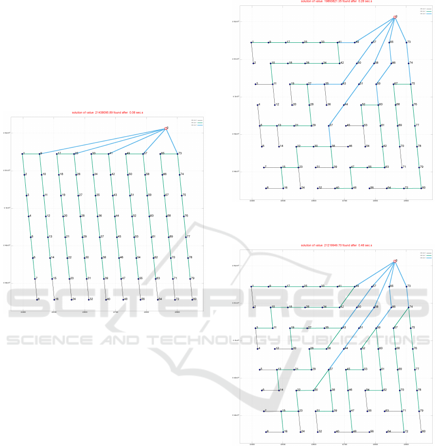
In Figure 4 the case of Horns Rev 3 with cable set
cb04 is shown.
1
It is seen that both the structure of the
cable routing and the usage of thicker cables (green in
the figure) increases in the loss-optimized layout.
1
This is a preliminary layout from Vattenfall, not neces-
sarily reflecting the final layout.
ICORES 2017 - 6th International Conference on Operations Research and Enterprise Systems
114
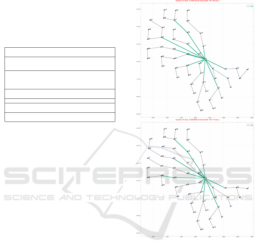
Table 5: Increase in the initial investment and long term
savings for our test instances (Net Present Value). The first
two columns denote the wind farm and possible cable types.
The next column shows how much the investment is in-
creased in the layout taking cable losses into account. In all
test cases this amount is paid back in 25 years, and the addi-
tional savings by using the lifetime-optimized cable layout
are shown in the last column.
wind farm cable set increase in savings
initial investment [Ke] in 25y [Ke]
Horns Rev 1 cb01 1 23
cb02 24 60
cb05 103 56
Kentish Flats cb01 2 3
cb02 1 4
cb04 19 8
cb05 5 1
Ormonde cb03 9 0
cb04 19 16
DanTysk cb01 115 21
Thanet cb04 15 92
cb05 1 19
Horns Rev 3 cb04 42 172
cb05 682 208
In this case the loss-optimized layout is 41 Ke
more expensive at construction time (with respect to
the CAPEX optimized layout). Nevertheless, in 25
years, this amount is paid back and another 172 Ke
are saved (NPV).
We now try to investigate how the optimizer is re-
structuring the layout in order to have savings in the
long run. As already noticed, every wind farm is dif-
ferent, so one cannot define a rule of thumb to design
a good cable routing. Nevertheless, observing our
layouts, we noticed a different proportion in the usage
of the cable types (black and green in the figures). In
particular, all the CAPEX solutions minimize the use
of the expensive cables: looking only at the immedi-
ate costs, it is always preferable to go for the cheap-
est cable when possible, even creating longer connec-
tions. When optimizing considering losses, instead,
cables with less resistance become more appealing,
even if they are more expensive. In the Horns Rev 1
instance, for example, going from CAPEX optimized
to lifetime-optimized the usage of type 1 cables de-
creases (from 55.5% of the total length to 40.3%) and
the usage of type 2 cables increases (from 44.5 to
59.7%).
In Table 6 we report the cable usage (percentage
of the total cable length) for all our test-bed solutions.
All in all, it can be observed from our results on
real-world instances that in most cases it is convenient
to invest in cables with lower resistance. The cable
route and the type of cable selection for each connec-
tion is not an obvious choice and an optimization tool
is necessary to determine it.
Figure 4: Optimized cable routing for Horns Rev 3, using
cable set cb04. We imposed that cable type 2 can support
5 turbines only twice. The top layout is optimized only on
CAPEX, the second is also considering power losses.
4.3 Bi-objectivity Tests
As discussed in Subsection 2.2, our problem has to
balance between two opposite objectives: minimiz-
ing immediate costs and minimizing revenue losses
in the long run. As we have seen in the previous tests,
these two objectives are not always aligned since the
more expensive cables have lower resistances (so less
losses). The balancing factor between the two objec-
tives is K
euro
, that represents the price of energy (Net
Present Value). Setting K
euro
to zero, for example,
means that there is no revenue from selling energy,
therefore it does not matter to have losses, but it is
On the Impact of using Mixed Integer Programming Techniques on Real-world Offshore Wind Parks
115

Table 6: Analysis on the usage of different types of cables
when optimizing considering or not considering losses. The
last three columns report the usage of the different cable
types as percentage of the total cable length of that layout.
ID wind farm cable set opt mode length per cable type [%]
Type 1 Type 2 Type 3
1 Horns Rev 1 cb01 capex 55.1 40.1 4.8
2 lifetime 53.6 41.7 4.7
3 cb02 capex 57.4 42.6
4 lifetime 44.1 55.9
5 cb05 capex 100.0 0.0
6 lifetime 87.7 12.3
7 Kentish Flats cb01 capex 66.4 33.6 0.0
8 lifetime 66.1 33.9 0.0
9 cb02 capex 66.4 33.6
10 lifetime 60.8 39.2
12 cb04 capex 90.1 9.9
13 lifetime 90.1 9.9
14 cb05 capex 95.6 4.4
15 lifetime 95.6 4.4
16 Ormonde cb03 capex 69.6 30.4
17 lifetime 76.7 23.3
18 cb04 capex 66.9 33.1
19 lifetime 67.4 32.6
20 DanTysk cb01 capex 39.0 19.4 41.7
21 lifetime 38.7 22.5 38.8
26 Thanet cb04 capex 86.3 13.7
27 lifetime 82.7 17.3
28 cb05 capex 71.9 28.1
29 lifetime 71.9 28.1
30 Horns Rev 3 cb04 capex 57.4 42.6
31 lifetime 60.7 39.3
32 cb05 capex 51.8 48.2
33 lifetime 52.6 47.4
instead important only to minimize immediate costs.
This corresponds to the case that we called ”CAPEX
optimized” in the previous tests. On the contrary, set-
ting K
euro
to a high value, implies that big revenue
can be earned selling more energy, so it is very im-
portant to minimize losses (whatever initial costs this
could imply). The balance between the two objec-
tives, in practice, is set by defining the parameter K
euro
for the specific project of interest. This is a value
known by the designer, and varies from project to
project. A realistic value for K
euro
has been used in
the tests of the previous subsection (this value consid-
ered WACC, subsidies for 10 years of operations and
estimated market price). Nevertheless, one could be
interested in studying how the balance between im-
mediate costs and long term costs varies when vary-
ing K
euro
. As a practical example, one could be in-
terested in optimizing CAPEX and losses at the same
time, but being sure to pay off the extra investment
in a short time. We considered, in this test, Horns
Rev 3 with cable set cb04. For K
euro
= 0 we have our
CAPEX solution of Figure 4 (top), for K
euro
= 690
e/MWh we have our life-time losses optimized so-
lution of Figure 4 (bottom). Company experts es-
timated 690 e/MWh to be a realistic value for the
energy earning over 25 years of operation (expected
lifetime of a wind park). We asked them to recom-
pute this value assuming that we want a return of
investment in a shorter time. They recomputed it
to be K
euro
= 176 for two years, K
euro
= 252 for 3
years, K
euro
= 321 for 4 years, and K
euro
= 386 for
5 years. Setting our balancing factor K
euro
to these
values translates in imposing that extra CAPEX cost
will be paid back in 2, 3, 4 or 5 years, respectively.
We recomputed the cable costs according to these dif-
ferent values of K
euro
and re-optimized the layout ac-
cordingly. Once the optimized layouts were found,
we re-evaluated them with K
euro
= 0 to evaluate their
CAPEX costs and K
euro
= 690 to estimate their cost
in 25 years. Table 7 shows these figures. For K
euro
higher than 321 e/MWh the layout is not changing
any more. This means that in the lifetime optimized
solution (K
euro
= 690) all the additional CAPEX costs
were actually paid back in 4 years of operation. In
Figure 5 we plot the values from Table 7: the value of
the different layouts is decomposed into its CAPEX
(x axis) and lifetime-cost part (y axis). The first point
(the “+” on the leftmost extreme) represents the value
for the CAPEX optimized solution (K
euro
= 0): it has
the lowest immediate cost, but the highest cost on the
long run. Proceeding from left to right, the next “+”s
represent the solutions optimized over 2, 3, 4 and 5
years respectively. From 4 years on, the layout is not
changing any more, and equals the solution optimized
on the park lifetime (K
euro
= 690), therefore all these
layouts are represented at the same coordinates in the
plot in Figure 5.
Table 7: Bi-objective analysis for Horns Rev 3 with cable
set cb04: changing solutions varying the parameter K
euro
.
K
euro
immediate cost total lifetime revenue loss due
[ke] cost [ke] to power losses [ke]
0 47283 52663 5379
176 47291 52551 5259
252 47309 52508 5199
321 47325 52490 5165
386 47325 52490 5165
690 47325 52490 5165
5 CONCLUSIONS
In this paper we used a Mixed Integer Linear Pro-
gramming (MILP) approach to optimize inter-array
offshore cable routing considering both the immedi-
ate cost of the cables and their power losses during the
wind farm lifetime. We proved the importance of us-
ing sophisticated optimization tools for this problem.
We compared the optimized solution with an exist-
ing cable layout, proving that millions of euros can be
saved in the given case. We also performed different
what-if analyses taking power losses into considera-
tion. Thanks to our optimization methods, we have
been able, for the first time, to quantify the impact of
considering losses when designing the cable connec-
tion of a wind farm. We performed these analyses on
ICORES 2017 - 6th International Conference on Operations Research and Enterprise Systems
116
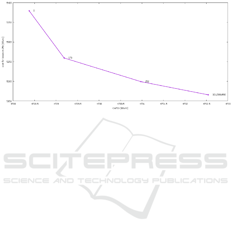
Figure 5: Bi-objective analysis from Table 7. Each “+” corresponds to a layout optimized for a given value of K
euro
(specified
beside each “+”) and its coordinates correspond to its immediate cost (x axis) and costs in 25years (y axis). The layouts
optimized with K
euro
= 321, 386, and 690 are the same.
a number of real-world instances, analysing the be-
haviour of the solutions. In general, we observed that
it is convenient to invest in cables with less resistance
in order to reduce power losses, even if these cables
are more expensive at construction time. We used our
testbed to evaluate the profitability of the new solu-
tions, both in terms of CAPEX and revenue in the
long term. Finally, we performed a Pareto optimal-
ity analysis by varying the balancing parameter K
euro
.
This corresponds to giving more or less importance to
power losses in the objective function, and is of great
importance for designers. In this way, indeed, they
can evaluate the return of investment and the impact
of their assumptions on the long-term energy price,
when designing their cable routing.
ACKNOWLEDGEMENTS
This work was supported by Innovation Fund Den-
mark. The authors would like to thank Jesper Runge
Kristoffersen, Kenneth Skaug, Thomas Hjort and Iu-
lian Vranceanu from Vattenfall BA Wind who helped
in defining the cable routing constraints and the cable
losses.
REFERENCES
Bauer, J. and Lysgaard, J. (2015). The offshore wind farm
array cable layout problem: a planar open vehicle
routing problem. Journal of the Operational Research
Society, (66.3):360–368.
Berzan, C., Veeramachaneni, K., McDermott, J., and Reilly,
U. O. (2011). Algorithms for cable network design
on large-scale wind farms. Technical report. Mas-
sachusetts Institute of Technology.
Cerveira, A., Sousa, A. D., Pires, E. J. S., and Baptista,
J. (2016). Optimal cable design of wind farms: The
infrastructure and losses cost minimization case. IEEE
Transactions on Power Systems, (31.6):4319 – 4329.
Dutta, S. (2012). Data Mining and Graph Theory Focused
Solutions to Smart Grid Challenges. PhD thesis, Uni-
versity of Illinois.
Dutta, S. and Overbye, T. J. (2011). A clustering based wind
farm collector system cable layout design. In Power
and Energy Conference at Illinois (PECI), pages 1–6.
Fagerfjall, P. (2010). Optimizing wind farm layout: more
bang for the buck using mixed integer linear program-
ming.
Fischetti, M. and Pisinger, D. (2016). Optimizing wind farm
cable routing considering power losses. Technical re-
port. Danish Technical University.
Gonzlez, J., Payn, M., Santos, J., and Gonzlez-Longatt, F.
(2014). A review and recent developments in the op-
timal wind-turbine micro-siting problem. Renewable
and Sustainable Energy Reviews, (30):133–144.
Gonzlez-Longatt, F. M. and Wall, P. (2012). Optimal
electric network design for a large offshore wind
farm based on a modified genetic algorithm approach.
IEEE Systems Journal, (6.1):164–172.
Hertz, A., Marcotte, O., Mdimagh, A., Carreau, M., and
Welt, F. (2012). Optimizing the design of a wind farm
collection network. Information Systems and Opera-
tional Research, (50.2):95–104.
Kristoffersen, J. and Christiansen, P. (2003). Horns rev off-
On the Impact of using Mixed Integer Programming Techniques on Real-world Offshore Wind Parks
117

shore windfarm: Its main controller and remote con-
trol system. Wind Engineering, (27.5):351–359.
Li, D., He, C., and Fu, Y. (2008). Optimization of internal
electric connection system of large offshore wind farm
with hybrid genetic and immune algorithm. In Third
International Conference on Electric Utility Dereg-
ulation and Restructuring and Power Technologies
(DRPT2008), pages 2476–2481.
Pillai, A., Chick, J., Johanning, L., and Laleu, M. K. V. D.
(2015). Offshore wind farm electrical cable layout op-
timization. Engineering Optimization, (47.12):1689–
1708.
Zhao, M., Chen, Z., and Blaabjerg, F. (2009). Optimisa-
tion of electrical system for offshore wind farms via
genetic algorithm. IET Renewable Power Generation
3, (3.2):205–216.
ICORES 2017 - 6th International Conference on Operations Research and Enterprise Systems
118
