A Single-source Weber Problem with Continuous Piecewise Fixed Cost
Gabriela Iriarte, Pablo Escalona, Alejandro Angulo and Raul Stegmaier
Department of Industrial Engineering, Universidad T´ecnica Federico Santa Mar´ıa, Valpara´ıso, Chile
Keywords:
Weber Problem, Fixed Costs, Delaunay Triangulation, Kriging Interpolation.
Abstract:
This paper analyzes the location of a distribution center in an urban area using a single-source Weber problem
with continuous piecewise fixed cost to find a global optimal location. The fixed cost is characterized by
a Kriging interpolation method. To make the fixed cost tractable, we approximate this interpolation with
a continuous piecewise function that is convex in each piece, using Delaunay triangulation. We present a
decomposition formulation, a decomposition conic formulation and a conic logarithmic disaggregated convex
combination model to optimally solve the single-source Weber problem with continuous piecewise fixed cost.
Although our continuous approach does not guarantee the global optimal feasible location, it allows us to
delimit a zone where we can intensify the search of feasible points. For instances we tested, computational
results show that our continuous approach found better locations than the discrete approach in 23.25% of the
instances and that the decomposition formulation is the best one, in terms of CPU time.
1 INTRODUCTION
The location of a distribution center (DC) in an ur-
ban area, considering the transportation and installa-
tion costs, can be treated as an uncapacitated facility
location problem (UFLP) or as a Weber problem with
fixed cost. It is known that the solution of the UFLP is
feasible but not necessarily optimal, due to the use of
an incomplete set of possible locations. On the other
hand, the Weber problem with fixed cost gives an op-
timal location probably not feasible.
This paper analyzes the installation of a single DC
in an urban area, using the single-source Weber prob-
lem with fixed cost to find an optimal location that al-
lows us to delimit a zone around the optimal location
previously found, but smaller than the original one.
This way, we can focus the search of feasible points,
obtaining a more reliable and complete set of possible
locations such that, when an UFLP is applied, we find
the optimal feasible location.
To the best of our knowledge,fewpapers deal with
the inclusion of the fixed costs into the Weber prob-
lem. Fixed costs have been considered as a constant
cost for all the plane (Brimberg et al., 2004), as zone
dependent with a constant cost in a specific convex
polygon (Brimberg and Salhi, 2005),(Hosseininezhad
et al., 2015), or as a proportion between the fixed cost
of two zones and their relative distance, (Luis et al.,
2015). To consider that a plane can be partitioned in a
finite set of convex polygons, each one with constant
fixed costs, is considered a good first approximation
to characterize the variating nature of this cost. In this
paper we propose that the fixed cost on each convex
polygon is a function of its vertices, allowing us to
better model the fixed costs in an urban area.
The objective of this paper is to find the best for-
mulation to locate a single DC in an urban area, where
the fixed costs depend on the location in a continu-
ous way. The fixed cost function is characterized by
a Kriging interpolation method using a set of nodes
where the cost is known. To make the formulation
tractable, we approximate the interpolation with a
continuous piecewise function that is convex in each
piece. This is constructed through a convex combi-
nation of the vertices of a mesh created with a De-
launay triangulation. The sinlge-source Weber prob-
lem with continuous piecewise fixed cost is formu-
lated as an MINLP problem. We take advantage of
the problem’s structure to propose three solution ap-
proaches. The first approach considers a conic re-
formulation of the single-source Weber problem with
continuous piecewise fixed cost using a logarithmic
disaggregated convex combination model. The sec-
ond consists of a decomposition method, where we
solve a non-linear convex problem for each Delaunay
triangle, and using complete enumeration we deter-
mine the optimal solution. The last one, consider a
conic reformulation for each sub-problem of the sub-
Iriarte G., Escalona P., Angulo A. and Stegmaier R.
A Single-source Weber Problem with Continuous Piecewise Fixed Cost.
DOI: 10.5220/0006191003370344
In Proceedings of the 6th International Conference on Operations Research and Enterprise Systems (ICORES 2017), pages 337-344
ISBN: 978-989-758-218-9
Copyright
c
 2017 by SCITEPRESS – Science and Technology Publications, Lda. All rights reserved
337

sequent decomposition formulation. Each approach
was implemented in a series of experiments to com-
pare their performance in CPU time.
The main contributions of this paper are: (i) a
new way to represent the fixed costs in an urban area
and (ii) to identify the best solution approach for the
single-source Weber problem with continuous piece-
wise fixed cost.
The paper is organized as follows: Section 2
presents our related work. Section 3 presents a
single-source Weber problem with continuous piece-
wise fixed cost. Section 4 presents three different ap-
proaches to solve the problem defined in the previous
section. Section 5 presents some experimental results
for all the different approaches. Our conclusions and
highlights are presented in section 6.
2 RELATED WORK
The continuous location problem for a single-source
or single-source Weber problem, described in We-
ber and Friedrich (1929), has been extensively stud-
ied. To find the solution there are different ap-
proaches: a one-point iterative method better known
as the Weiszfeld algorithm (Weiszfeld and Plastria,
2009), a unified cutting plane method (Plastria, 1987),
a dual method (Planchart and Hurter, 1975), a primal-
dual algorithm involving mixed norms (Michelot and
Lefebvre, 1987), or a primal-dual potential reduction
algorithms with the problem formulated in conic form
(Xue and Ye, 1997). A comprehensive review of the
Weber problem can be found in Drezner et al. (2002).
The multi-source Weber problem, or location-
allocation problem, is an NP-hard problem (Megiddo
and Supowit, 1984). There are few heuristics that
solve it to optimality but they work only in small prob-
lems (Cooper, 1972), (Sherali et al., 2002), (Chen
et al., 1998). For the heuristic approach to solve
the problem to near optimum, there are more pub-
lications: Cooper (1964) explored different algo-
rithms with computational experiments. The alter-
nating location-allocation heuristic is used by Cooper
(1972). The method used by Bongartz et al. (1994)
relaxes the binary constraints on the allocations, and
solves both location and allocation simultaneously.
An approach based on a nonlinear second-order cone
program reformulation is found in Chen et al. (2011).
The approach to use the discrete models in solving
the continuous location-allocation problems is widely
used by Hansen et al. (1998), Brimberg et al. (2014),
and others. For this, a survey in the p-median problem
with the aim in procedures based on metaheuristics
rules (Mladenovic et al., 2007) is useful. For a survey
on the multi-source Weber problem there is Brimberg
et al. (2000) and Brimberg et al. (2008).
The inclusion of the fixed cost to the Weber prob-
lem has little reviews, there are four papers to the best
of our knowledge. First it is included as a constant
cost for all plane in Brimberg et al. (2004). Later,
in Brimberg and Salhi (2005), it was extended to
a zone-dependent fixed cost, where zones are non-
overlapping convex polygons with a constant fixed
cost for each zone. In Hosseininezhad et al. (2015) is
developed a metaheuristic Cross Entropy for a contin-
uous location problem, with an fixed cost depending
on the zone and on the facility to install. And Luis
et al. (2015), proposed a multi-source Weber problem
with capacity and zone-dependent fixed cost using the
second-order Voronoi regions.
In general, data gathering is expensive in terms of
monetary and time-consuming costs (Helbich et al.,
2013). Therefore, there is a necessity to estimate
the land values in unvisited locations, as geostatis-
tical methods Luo (2004), Cellmer et al. (2014).
Here, we use a Kriging method of interpolation
(Oliver and Webster, 1990). This method was rec-
ommended over other interpolation approaches in
Anselin and Le Gallo (2006) and Fern´andez-Avil´es
et al. (2012), in an air quality and pollution stud-
ies, respectively. The possibilities and limitations of
geostatistical methods to approximate the land values
are discussed in Cellmer (2014). A comparison be-
tween Kriging methods for the real estate market is
discussed in Kuntz and Helbich (2014). The Kriging
interpolation is used to find the value of land for dif-
ferent cities by Liang and Yi (2012), Hu et al. (2015),
Larraz and Poblacin (2013).
In summary, there are few previous works on
single-source and multi-source Weber problem that
include a second order cone formulation and, to the
best of our knowledge, only one paper presents a so-
lution approach. The few papers that include fixed
costs make a simplistic representation of them that do
not reflect their variations in an urban area. Unlike
them, we make a more realistic representation of the
fixed costs, considering different possible approaches
for the Weber problem with fixed costs.
3 MODEL FORMULATION
3.1 Single-source Weber Problem with
Continuous Piecewise Fixed Costs
The generalized single-source Weber problem with
fixed costs considers the localization of a single
ICORES 2017 - 6th International Conference on Operations Research and Enterprise Systems
338

source with coordinates ( ¯x, ¯y) ∈ R
2
. This source must
supply a set J of customers with known coordinates,
(xc
j
, yc
j
) for every j ∈ J. Let f( ¯x, ¯y) be the fixed cost
incurred when the source is installed in ( ¯x, ¯y). Let w
j
be the the expected demand weighted by the trans-
portation ratios, for all j ∈ J. The problem is to deter-
mine the optimal location for the single source such
that the transportation and the fixed costs are mini-
mized. The generalized single-source Weber problem
with fixed costs can be expressed as follows:
min
( ¯x, ¯y)
∑
j∈J
w
j
q
( ¯x− xc
j
)
2
+ ( ¯y− yc
j
)
2
+ f( ¯x, ¯y) (1)
s.t. ( ¯x, ¯y) ∈ R
2
(2)
We consider a convenient set I of nodes with
known information of their fixed costs, C
i
, and their
coordinates, (xi
i
, yi
i
), for every i ∈ I. In our paper, the
way to address the fixed costs is by applyinga Kriging
interpolation method and defining a continuous func-
tion for the cost in every point of the convex hull of
I. This cost function is not simple and could not be
convex. To make the continuous fixed cost function
tractable, we are going to approximate the Kriging in-
terpolation with a piecewise function that is convexin
each piece. For this, we partition the convex hull of
I through a polyhedral mesh and defined the continu-
ous piecewise fixed cost function as the convex com-
bination of the vertices of the mesh. To the best of our
knowledge, it is better to use the smallest subset of in-
formation nodes possible with empty interior to create
the polyhedra, i.e, using Delaunay triangulation.
We applied a Delaunay triangulation over the set
I obtaining a set K of triangles; each triangle k-th
will be denoted as P
k
, with P
k
= {(x, y) ∈ R
2
|(x, y) =
∑
3
l=1
λ
k
l
(x
k
l
, y
k
l
),
∑
3
l=1
λ
k
l
= 1, ∀λ
k
l
: λ
k
l
≥ 0}, where
(x
k
1
, y
k
1
), (x
k
2
, y
k
2
) and (x
k
3
, y
k
3
) are the vertices of
the k-th triangle and C
k
1
, C
k
2
, C
k
3
their fixed cost. We
have λ
k
l
as the convex combination vector for the ver-
tices of the triangle k ∈ K and l = 1, 2, 3 the vertices of
the triangle. The set of all possible locations,
S
k∈K
P
k
,
can be non-convex if we clean the areas where we can
not install, as a lake or a strictly residential area.
Given the above, the facility’s location can be ex-
pressed as ( ¯x, ¯y) =
∑
k∈K
∑
3
l=1
λ
k
l
(x
k
l
, y
k
l
) and its fixed
cost as a convexcombination of the vertices of the tri-
angles’s costs,
∑
k∈K
∑
3
l=1
C
T
k
l
λ
k
l
. Let Z
k
be a binary
variable that forces the installation to be in only one
triangle, being 1 if it is installed in the k-th triangle
and 0 if it is not.
We can formulate the single-source Weber prob-
lem with continuous piecewise fixed cost as follows:
Problem (P0):
min
Z,λ
∑
k∈K
3
∑
l=1
C
k
l
λ
k
l
+ Z
k
∑
j∈J
w
j
v
u
u
t
(
∑
k∈K
3
∑
l=1
λ
k
l
x
k
l
− xc
j
)
2
+ (
∑
k∈K
3
∑
l=1
λ
k
l
y
k
l
− yc
j
)
2


(3)
s.t.
3
∑
l=1
λ
k
l
= Z
k
, ∀k ∈ K (4)
∑
k∈K
Z
k
= 1 (5)
λ
k
l
≥ 0, ∀l ∈ {1, 2, 3}, k ∈ K (6)
Z
k
∈ {0, 1}, ∀k ∈ K (7)
In what follows, we present different ways to
solve the problem (P0).
4 SOLUTION APPROACH
We consider three distinct solution approaches for
(P0). For the first approach, we use a monolithic re-
formulation of (P0). The second approach considers
a decomposition of (P0) by fixing the variable Z and
solving the sub-problem generated; we evaluated all
the possible values of Z. The last approach considers
a conic reformulation of the previous sub-problems.
4.1 Conic Logarithmic Disaggregated
Convex Combination Model
Now, we reformulate (P0) in two steps. First, we for-
mulate the problem as a Conic Quadratic Non Lin-
ear problem (CQNLP). Afterwards, using the log-
arithmic disaggregated convex combination model
(Vielma et al., 2010), we efficiently solve the contin-
uous piecewise fixed cost function.
Next, we formulate the problem (P0) as a CQNLP
in order to eliminate the square root terms. First
we introduce one set of nonnegative continuous vari-
ables, d
j
, to represent the square root term in:
d
j
=
v
u
u
t
(
3
∑
l=1
x
k
l
λ
k
l
− xc
j
)
2
+ (
3
∑
l=1
y
k
l
λ
k
l
− yc
j
)
2
, ∀ j ∈ J
(8)
d
j
≥ 0, ∀ j ∈ J (9)
A Single-source Weber Problem with Continuous Piecewise Fixed Cost
339

For simplicity, we can add two more sets of auxil-
iary variables, v
j
and r
j
, leaving (8) as:
d
2
j
= z
2
j
+ w
2
j
, ∀ j ∈ J (10)
v
j
=
3
∑
l=1
x
k
l
λ
k
l
− xc
j
, ∀ j ∈ J (11)
r
j
=
3
∑
l=1
y
k
l
λ
k
l
− yc
j
, ∀ j ∈ J (12)
Because the nonnegative variables d
j
are intro-
duced in the objective function of (P0) with positive
coefficients, and this problem is a minimization prob-
lem, the equation can be further relaxed as the follow-
ing inequalities:
d
2
j
≥ v
2
i
+ r
2
i
, ∀ j ∈ J (13)
Note that the constraints (9) and (13) define
second-order cone constraints. The problem (P0) can
be expressed as the following conic problem:
Problem (CP0):
min
Z,λ,d,v,r
∑
k∈K
(Z
k
∑
j∈J
w
j
d
j
+
3
∑
l=1
C
k
l
λ
k
l
) (14)
s.t. (4), (5), (6), (7), (9), (11), (12), (13)
The logarithmic disaggregated convex combina-
tion model consists in replacing the piecewise func-
tion f ( ¯x, ¯y) for its epigraph epi( f) and setting the co-
ordinate ( ¯x, ¯y) to be contained by one and only one
of the domains of f. For a minimization, solving the
function f is equivalent to solving epi( f). To con-
struct a model with the least number of binary vari-
ables and constraints, we identify each triangle with
a binary vector in {0, 1}
⌈log
2
|K|⌉
through an injective
function B : K → {0, 1}
⌈
log
2
|K|⌉
and use ⌈log
2
|K|⌉ bi-
nary variables, m ∈ {0, 1}
⌈log
2
|K|⌉
, to ensure that the
coordinates are in only one triangle. Let Q be epi( f).
Using the logarithmic disaggregated convex com-
bination model and a second order cone formulation
to reformulate (P0), leaves the following:
Problem (DlogCP0):
min
λ,m,d,Q,v,r
∑
j∈J
w
j
d
j
+ Q (15)
s.t.
∑
k∈K
3
∑
l=1
C
k
l
λ
k
l
≤ Q (16)
∑
k∈K
3
∑
l=1
λ
k
l
= 1 (17)
∑
k∈K
+
(B,t)
3
∑
l=1
λ
k
l
≤ m
t
, ∀t ∈ T(K) (18)
∑
k∈K
0
(B,t)
3
∑
l=1
λ
k
l
≤ (1− m
t
), ∀t ∈ T(K)
(19)
λ
k
l
≥ 0 ∀l ∈ 1, 2, 3, k ∈ K (20)
m
t
∈ {0, 1} ∀t ∈ T(K) (21)
(9), (11), (12), (13)
where B : K → {0, 1}
⌈log
2
|K|⌉
is any injective func-
tion, K
+
(B, t) = {k ∈ K : B(k)
t
= 1}, K
0
(B, t) = {k ∈
K : B(k)
t
= 0} and T(K) = {1, . . . , ⌈log
2
|K|⌉}. This
problem is a mixed integer conic quadratic nonlinear
problem with a linear objective function and can be
solved by solvers like GUROBI, CPLEX or MOSEK.
4.2 Decomposition Formulation
From the problem (P0), we can observe that the vari-
ables λ and Z are related in only one constraint. And,
fixing the variable Z, the problem is separable in |K|
sub-problems where we force the localization of the
DC to be in the k-th Delaunay triangle, i.e., forcing
Z
k
= 1 and Z
k
′
= 0 for all k
′
∈ K \ k. Then the k-th
sub-problem can be written as:
Sub-Problem (SP0(k)):
min
λ
k
∑
j∈J
w
j
q
( ¯x− xc
j
)
2
+ ( ¯y− yc
j
)
2
+
3
∑
l=1
C
k
l
λ
k
l
(22)
s.t.
3
∑
l=1
λ
k
l
= 1 (23)
λ
k
l
≥ 0 , ∀l ∈ {1, 2, 3} (24)
This sub-problem (SP0(k)) is a convex nonlinear
problem with linear constraint and can be efficiently
solved by MINOS or IPOPT solvers.
Let λ
k
∗
be the optimal solution of the problem
(SP0(k)); FO
(SP0(k))
(λ
k
∗
) be the optimal cost of the
objective function in the problem (SP0(k)), and let
(
¯
λ,
¯
Z) be the optimal solution of the problem (P0).
The optimal solution for the (P0) problem is the best
solution for all of the sub-problems (SP0(k)), i.e.
¯
λ =
λ
k
†
, where k
†
= argmin
k∈K
{FO
(SP0(k))
(λ
k
∗
)}. For
¯
Z,
the value of
¯
Z
k
= 1 for k = k
†
and
¯
Z
k
= 0 for every
other k.
4.3 Decomposition Conic Formulation
The squared root term in the objective function of
problem (SP0(k)) can give rise to difficulties in the
optimization procedure. Following the logic exposed
for the first approach, we reformulate (SP0(k)) as a
CQNLP, leaving the following conic problem:
ICORES 2017 - 6th International Conference on Operations Research and Enterprise Systems
340

Sub-Problem (SCP0(k)):
min
λ
k
,d,v,r
∑
j∈J
w
j
d
j
+
3
∑
l=1
C
k
l
λ
k
l
(25)
s.t. (23), (24), (9), (11), (12), (13)
The problem (SCP0(k)) can be trivially shown to
be equivalent to (SP0(k)), but it has now conic and
nonlinear constraints with a more simple linear objec-
tive function. The optimal solution for (P0) is the best
solution for all the sub-problems (SCP0(k)), equiva-
lently to the decomposition formulation.
The advantage of the CQNLP formulation is that
it can be solved directly using standard optimiza-
tion software packages such as CPLEX, GUROBI or
MOSEK.
5 COMPUTATIONAL STUDY
In this section, we present our numerical study and
its results. The main objectives of this computational
study is to show which solution approach has the best
performance in terms of CPU time, and to compare
them to an UFLP. To characterize the different ap-
proaches, we carried out 400 instances that we denote
test set. We also corroborate the installation of a sin-
gle DC in every instance with the UFLP.
All the problems were programmed using AMPL.
To solve the decomposition formulation we use the
solver MINOS. For (DlogCP0) and the decomposi-
tion conic formulation we solve it through CPLEX
solver. The Kriging interpolation method and the De-
launay triangulationwere made in MATLAB.The test
set were run on a PC with AMD FX 4,00 GHz pro-
cessor and 12 GB RAM, and the UFLP were run on a
PC with Intel i3 2,10 Ghz and 4 GB RAM.
5.1 Test Set
In order to determine which one has the best perfor-
mance in CPU time, we generated 100 experiments.
In each experiment, we fixed the number of customer
nodes and used 4 refinements of the triangulation.
Therefore, we have 400 instances. For simplicity, we
considered w
j
= 1, for any j ∈ J.
Each experiment has the same initial set of 100
information nodes, generated randomly. For a bet-
ter piecewise convex approximationof the continuous
fixed cost function, we proposed the following refine-
ment of the mesh. We consider the Delaunay triangu-
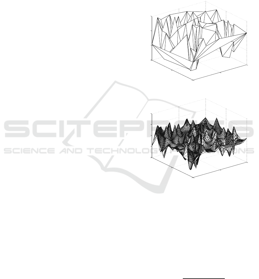
lation of the initial set of information nodes as the first
refinement, shown in figure 1. The second refinement
is generated by creating additional information nodes
where their location is at the center of the edge of ev-
ery triangle and their fixed cost is determined by the
Kriging interpolation. Then the Delaunay triangula-
tion is used over the original set I plus the additional
information nodes. The third and fourth refinements
are applied over the second and third triangulation, re-
spectively. In figure 2 the fourth refinement is shown.
0
50
100
0
50
100
0
2000
4000
6000
X
Y
Fixed Cost
Figure 1: First refinement.
0
50
100
0
50
100
0
2000
4000
6000
8000
X
Y
Fixed Cost
Figure 2: Fourth refinement.
We modified the number of customer nodes from
100 to 1000 customers, i.e., the first 10 experiments
have 100 customer nodes, the next 10 experiments
have 200 customer nodes, and so on. Each customer
location is obtained making random locations, i.e.,
where (xc
j
, yc
j
) ∈ ([0, 100], [0, 100]).
Figure 3 shows the performance profile based on
the performance ratio of the CPU time for each model
(Dolan and Mor´e, 2002). Considering that t
pm
is the
CPU time for solving the instance p by the model m,
we have the performance ratio:
r
pm
=
t
pm
min{t
pm
: m ∈ M}
,
where M = {DlogCP0, min
k∈K
{(SP0(k))},
min
k∈K
{(SCP0(k))}}.
A Single-source Weber Problem with Continuous Piecewise Fixed Cost
341

0
50
100
150
0.00 0.25 0.50 0.75 1.00
τ
Methods
min
k∈K
(SP0(k))
min
k∈K
(SCP0(k))
DlogCP0
P(r ≤ τ)
Figure 3: Performance Profile.
We observe in figure 3 that the best model
performance is the decomposition formulation, i.e.,
min
k∈K
{(SP0(k))}, because in 80% of the instances
has the lowest time, overcome by (DlogCP0), in less
than 20% of the instance. The decomposition formu-
lation has the best performance with the greater effi-
ciency, solving all the instances with a r  5.
There is a pattern in every refinement where
(DlogCP0) has the best performance in the instances
with a small set of customers nodes, and get outper-
formed by the decomposition formulation in the rest
of the instances. This is shown in table 1, where
it shows that the average speedup in the CPU time
of the decomposition formulation over (DlogCP0) is
greater than 1x for all the refinements in the instances
with |J| = 100. Considering the second and third re-
finement, (DlogCP0) is better, in average, for the in-
stances with |J| ≤ 200. For the fourth refinement,
(DlogCP0) is better in instances with |J| ≤ 300 and
with an average speedup of over 4x when |J| = 100.
Table 1: Average Speedup in CPU time of
min
k∈K
{(SP0(k))} over (DlogCP0).
Refinement
|J| First Second Third Fourth
100 1.556x 2.035x 2.808x 4.125x
200 0.574x 1.185x 1.548x 1.944x
300 0.382x 0.865x 0.840x 1.149x
400 0.320x 0.665x 0.697x 0.494x
500 0.258x 0.528x 0.470x 0.308x
600 0.301x 0.530x 0.410x 0.330x
700 0.226x 0.447x 0.416x 0.099x
800 0.214x 0.387x 0.385x 0.036x
900 0.184x 0.373x 0.367x 0.020x
1000 0.172x 0.309x 0.312x 0.012x
We obtain an average speedup of 7.98x and 7.72x
for the decomposition formulation over the decompo-
sition conic formulationand (DlogCP0), respectively.
Our numerical results show that the performance
from the conic formulations ((DlogCP0) and the de-
composition conic formulation) are sensible to the
size of the customer set. This is because the conic
formulations create |J| cones and 3|J| new variables,
so the problem grows faster than the number of cus-
tomers. For this reason, even that (DlogCP0) can bet-
ter handle a big set of information nodes, this only is
seen with a small set of customers.
The performance of the decomposition formula-
tion, shown in figure 3, is the most stable of the per-
formances of the three solution approaches, i.e., with
less difference in the extremes values of its perfor-
mance ratio. This indicates that if the decomposition
formulation does not have the best performance in an
instance, its CPU time is closer to the better one.
The average improvement in the objective func-
tion using the different refinements, compared with
the first refinement, are: 0.08% for the second, 0.74%
for the third, and 1.29% for the fourth refinement.
We can observe in table 1 that in instances
with small number of customers is better to use
(DlogCP0), considering that can have a speedup over
4x against the decomposition formulation, but it is
when the CPU times are lower. For example, in all
the instances with |J| = 100, although we have a bet-
ter average of CPU time with (DlogCP0), the worst
CPU time for the decomposition formulation does not
get over 250 seconds. Considering that the decom-
position formulation has a more stable performance
with the better overall average in CPU time, and be-
cause this solves a strategic decision, we recommend
to model the single source Weber problem with fixed
cost with the decomposition formulation.
5.2 Discrete Model: Uncapacitated
Facility Location Problem
The following experiments where made using the in-
stances previously described in the test set, consider-
ing the set of information nodes without the refine-
ments. We consider the information nodes as the dis-
crete set of possible locations, modelled by an UFLP.
In table 2 are the average and maximum percent-
age of the improvement in lowering the value of the
objective function of the single-source Weber prob-
lem with continuous piecewise fixed cost over the
UFLP, and the number of cases where this happened.
Table 2 shows, for the fourth refinement an aver-
age improvement of 1.42%. From the total of exper-
iments solved with the fourth refinement, the 67% of
ICORES 2017 - 6th International Conference on Operations Research and Enterprise Systems
342

Table 2: Percentage of improvement for the continuous
model over the UFLP.
Refinement
First Second Third Fourth
Average 0.13% 0.21% 0.86% 1.42%
Max 1.62% 5.80% 16.83% 18.58%
N
◦
Cases 27 8 25 33
the instances have the same result as the UFLP. But
in the 33% where they are different, the average im-
provement is of 4.297%.
The better solutions found in 23.25% of the in-
stances with the single-source Weber problem over
the UFLP is because the UFLP only consider the in-
formation nodes as possible locations and not always
is consider the global optimum in that set. With the
inclusion of more information nodes, i.e. closer to
reality, the average savings and the number of better
cases tend to grow.
We also observed that in all the instances only one
facility is installed. This is in accordance to say that,
in an urban area, the fixed cost of an extra DC tends
to be bigger than the savings in transportation.
6 CONCLUSIONS
This paper analyses the problem of locating a single
DC in an urban area considering the fixed and trans-
portation costs using a single-source Weber problem
with continuous piecewise fixed cost. The fixed cost
is characterized by a Kriging interpolation method.
Using a Delaunay triangulation, we make the fixed
cost function convex and tractable. We propose
and evaluate three solution approaches to optimally
solve the single-source Weber problem with contin-
uous piecewise fixed cost: (i) decomposition formu-
lation, (ii) decomposition conic formulation, and (iii)
logarithmic disaggregated convexcombination model
with a conic formulation.
In the instances we tested, in 23.25% of the
time, a better solution is found with the single-
source Weber problem with continuous piecewise
fixed cost than with the UFLP. We observe two pos-
sible explanations:(i) the set I is complete, and there-
fore, the solution of the Weber problem is unfeasible,
and (ii) the set I is incomplete and requires a more
thorough search of feasible locations over the urban
area, i.e., the UFLP could have found a sub-optimal
solution. To ensure a complete set I in an urban area
is expensive and almost impossible. It is possible to
improve with the continuous approach, the set of fea-
sible locations focusing in a reduced section of the
urban area around the optimal location found, where
it is more probable to find the optimal feasible loca-
tion, thus reducing the search effort of feasible points.
With this, we can apply an UFLP over the new set I.
The computational results show that the best ap-
proach for the single-source Weber problem with con-
tinuous piecewise fixed cost, in terms of average CPU
time, is the decomposition method, with an average
speedup of 7.98x and 7.72x over the decomposition
conic method and the conic monolithic reformulation,
respectively. The first approach has the best perfor-
mance and can better handle a bigger set of informa-
tion nodes only with a small number of customers,
but this happens in the instances where the difference
between the CPU times are smaller.
There are a number of questions and issues left for
future research, such as: (i) to apply some Weizfield-
like algorithm to improve the performance of the
decomposition formulation, given that that was the
best one, (ii) to use the formulation of a stochastic
model of the single-source Weber problem with fixed
cost using the variance of the Kriging interpolation
method, (iii) to consider a location-routing problem,
and (iv) the extension to a multi-source Weber prob-
lem with continuous dependent fixed cost considering
the best solution approach we obtain.
REFERENCES
Anselin, L. and Le Gallo, J. (2006). Interpolation of air
quality measures in hedonic house price models: spa-
tial aspects. Spatial Economic Analysis, 1(1):31–52.
Bongartz, I., Calamai, P. H., and Conn, A. R. (1994). A pro-
jection method forl p norm location-allocation prob-
lems. Mathematical Programming, 66(1):283–312.
Brimberg, J., Drezner, Z., Mladenovic, N., and Salhi, S.
(2014). A new local search for continuous loca-
tion problems. European Journal of Operational Re-
search, 232(2):256–265.
Brimberg, J., Hansen, P., Mladenovic, N., and Salhi, S.
(2008). Survey of solution methods for the continuous
location-allocation problem. International Journal of
Operations Research, 5(1):1–12.
Brimberg, J., Hansen, P., Mladenovic, N., and Taillard,
E. D. (2000). Improvements and comparison of
heuristics for solving the uncapacitated multisource
weber problem. Operations Research, 48(3):444–460.
Brimberg, J., Mladenovic, N., and Salhi, S. (2004). The
multi-source weber problem with constant opening
cost. Journal of the Operational Research Society,
55(6):640–646.
Brimberg, J. and Salhi, S. (2005). A continuous location-
allocation problem with zone-dependent fixed cost.
Annals of Operations Research, 136(1):99–115.
Cellmer, R. (2014). The possibilities and limitations of geo-
statistical methods in real estate market analyses. Real
Estate Management and Valuation, 22(3):54–62.
A Single-source Weber Problem with Continuous Piecewise Fixed Cost
343

Cellmer, R., Belej, M., Zrobek, S., and
ˇ
Subic-Kovaˇc, M.
(2014). Urban land value maps a methodological ap-
proach. Geodetski vestnik, 58(3):535–551.
Chen, J.-S., Pan, S., and Ko, C.-H. (2011). A continua-
tion approach for the capacitated multi-facility weber
problem based on nonlinear socp reformulation. Jour-
nal of Global Optimization, 50(4):713–728.
Chen, P.-C., Hansen, P., Jaumard, B., and Tuy, H. (1998).
Solution of the multisource weber and conditional we-
ber problems by d.-c. programming. Operations Re-
search, 46(4):548–562.
Cooper, L. (1964). Heuristic methods fot location-
allocation problems. SIAM Review, 6(1):37–53.
Cooper, L. (1972). The transportation-location problem.
Operations Research, 20(1):94–108.
Dolan, E. D. and Mor´e, J. J. (2002). Benchmarking opti-
mization software with performance profiles. Mathe-
matical programming, 91(2):201–213.
Drezner, Z., Klamroth, K., Sch¨obel, A., and Wesolowsky,
G. O. (2002). 1 the weber problem.
Fern´andez-Avil´es, G., Minguez, R., and Montero, J.-M.
(2012). Geostatistical air pollution indexes in spatial
hedonic models: the case of madrid, spain. Journal of
Real Estate Research.
Hansen, P., Mladenovic, N., and Taillard, E. (1998). Heuris-
tic solution of the multisource weber problem as a
pmedian problem. Operations Research Letters, 22(2-
3):55–62.
Helbich, M., Jochem, A., M¨ucke, W., and H¨ofle, B. (2013).
Boosting the predictive accuracy of urban hedonic
house price models through airborne laser scanning.
Computers, environment and urban systems, 39:81–
92.
Hosseininezhad, S. J., Salhi, S., and Jabalameli, M. S.
(2015). A cross entropy-based heuristic for the capac-
itated multi-source weber problem with facility fixed
cost. Computers & Industrial Engineering, 83:151–
158.
Hu, S., Tong, L., Frazier, A. E., and Liu, Y. (2015). Urban
boundary extraction and sprawl analysis using landsat
images: A case study in wuhan, china. Habitat Inter-
national, 47:183–195.
Kuntz, M. and Helbich, M. (2014). Geostatistical mapping
of real estate prices: an empirical comparison of krig-
ing and cokriging. International Journal of Geograph-
ical Information Science, 28(9):1904–1921.
Larraz, B. and Poblacin, J. (2013). An online real estate
valuation model for control risk taking: A spatial ap-
proach. Investment Analysts Journal, 42(78):83–96.
Liang, H. and Yi, W. (2012). Effect of rent spatial distribu-
tion to urban business district planning. In Advanced
Materials Research, volume 374, pages 2001–2008.
Trans Tech Publ.
Luis, M., Salhi, S., and Nagy, G. (2015). A constructive
method and a guided hybrid grasp for the capacitated
multi-source weber problem in the presence of fixed
cost. Journal of Algorithms & Computational Tech-
nology, 9(2):215–232.
Luo, J. (2004). Modeling urban land values in a gis envi-
ronment. University of Wisconsin. Milwaukee, USA.
Megiddo, N. and Supowit, K. (1984). On the complexity
of some common geometric location problems. SIAM
Journal on Computing, 13(1):182–196.
Michelot, C. and Lefebvre, O. (1987). A primal-dual algo-
rithm for the fermat-weber problem involving mixed
gauges. Mathematical Programming, 39(3):319–335.
Mladenovic, N., Brimberg, J., Hansen, P., and Moreno-
Perez, J. A. (2007). The p-median problem: A sur-
vey of metaheuristic approaches. European Journal
of Operational Research, 179(3):927–939.
Oliver, M. A. and Webster, R. (1990). Kriging: a method
of interpolation for geographical information systems.
International Journal of Geographical Information
System, 4(3):313–332.
Planchart, A. and Hurter, A. P. J. (1975). An effi-
cient algorithm for the solution of the weber prob-
lem with mixed norms. SIAM Journal on Control,
13(3):650665.
Plastria, F. (1987). Solving general continuous single fa-
cility location problems by cutting planes. European
Journal of Operational Research, 29(1):98–110.
Sherali, H. D., Al-Loughani, I., and Subramanian, S.
(2002). Global optimization procedures for the
capacitated euclidean and l
p
distance multifacility
location-allocation problems. Operations Research,
50(3):433–448.
Vielma, J. P., Ahmed, S., and Nemhauser, G. (2010).
Mixed-integer models for nonseparable piecewise lin-
ear optimization: Unifying framework and extensions.
Operations Research, 58(2):303–315.
Weber, A. and Friedrich, C. J. (1929). Alfred Weber’s The-
ory of the Location of Industries. The University of
Chicago Press, Chicago, Illinois.
Weiszfeld, E. and Plastria, F. (2009). On the point for which
the sum of the distances to n given points is minimum.
Annals of Operations Research, 167(1):4–41.
Xue, G. and Ye, Y. (1997). An efficient algorithm for min-
imizing a sum of euclidean norms with applications.
SIAM Journal on Optimization, 7(4):1017–1036.
ICORES 2017 - 6th International Conference on Operations Research and Enterprise Systems
344