
A Hierarchical Tree Distance Measure for Classification
Kent Munthe Caspersen, Martin Bjeldbak Madsen, Andreas Berre Eriksen and Bo Thiesson
Department of Computer Science, Aalborg University, Aalborg, Denmark
{swallet, martinbmadsen}@gmail.com, {andreasb, thiesson}@cs.aau.dk
Keywords:
Machine Learning, Multi-class Classification, Hierarchical Classification, Tree Distance Measures, Multi-
output Regression, Multidimensional Scaling, Process Automation, UNSPSC.
Abstract:
In this paper, we explore the problem of classification where class labels exhibit a hierarchical tree structure.
Many multiclass classification algorithms assume a flat label space, where hierarchical structures are ignored.
We take advantage of hierarchical structures and the interdependencies between labels. In our setting, labels
are structured in a product and service hierarchy, with a focus on spend analysis. We define a novel distance
measure between classes in a hierarchical label tree. This measure penalizes paths though high levels in the
hierarchy. We use a known classification algorithm that aims to minimize distance between labels, given
any symmetric distance measure. The approach is global in that it constructs a single classifier for an entire
hierarchy by embedding hierarchical distances into a lower-dimensional space. Results show that combining
our novel distance measure with the classifier induces a trade-off between accuracy and lower hierarchical
distances on misclassifications. This is useful in a setting where erroneous predictions vastly change the
context of a label.
1 INTRODUCTION
With the increasing advancement of technologies de-
veloped to gather and store vast quantities of data, in-
teresting applications arise. Many kinds of business
processes are supported by classifying data into one
of multiple categories. In addition, as the quantity of
data grows, structured organizations of assigned cate-
gories are often created to describe interdependencies
between categories. Spend analysis systems are an ex-
ample domain where such a hierarchical structure can
be beneficial.
In a spend analysis system, one is interested in
being able to drill down on the types of purchases
across levels of specificity to aid in planning of pro-
curements. Such tools also provide processes to gain
insights in how much and to whom spending is going
towards, supporting spend visibility. For example, in
the UNSPSC
1
taxonomy, a procured computer mouse
would belong to the following categories of increasing
specificity: “Information Technology Broadcasting
and Telecommunications”, “Computer Equipment and
Accessories”, “Computer data input devices”, “Com-
puter mouse or trackballs”. For more information on
1
United Nations Standard Products and Services Code
R
,
a cross-industry taxonomy for product and service classifi-
cation.
the UNSPSC standard, see (Programme, 2016).
Many classification problems have a hierarchical
structure, but few multiclass classification algorithms
take advantage of this fact. Traditional multiclass clas-
sification algorithms ignore any hierarchical structure,
essentially flattening the hierarchy such that the clas-
sification problem is solved as a multiclass classifi-
cation problem. Such problems are often solved by
combining the output of multiple binary classifiers, us-
ing techniques such as One-vs-One and One-vs-Rest
to provide predictions (Bishop, 2006).
Hierarchical multiclass classification (HMC) algo-
rithms are a variant of multiclass classification algo-
rithms which take advantage of labels organized in a
hierarchical structure. Depending on the label space,
hierarchical structures can be in the shape of a tree
or directed acyclic graph (DAG). Figure 1 shows an
example of a tree-based label structure. In this paper,
we focus on tree structures.
Silla and Freitas (Silla and Freitas, 2011) de-
scribe hierarchical classification problems as a 3-tuple
hΥ, Ψ, Φi
, where
Υ
is the type of graph represent-
ing the hierarchical structure of classes,
Ψ
specifies
whether a datapoint can have multiple labels in the
class hierarchy, and
Φ
specifies whether the labeling
of datapoints only includes leaves or if nodes within
the hierarchy are included as well. Using this defini-
tion, we are concerned with problems of the form
502
Caspersen, K., Madsen, M., Eriksen, A. and Thiesson, B.
A Hierarchical Tree Distance Measure for Classification.
DOI: 10.5220/0006198505020509
In Proceedings of the 6th International Conference on Pattern Recognition Applications and Methods (ICPRAM 2017), pages 502-509
ISBN: 978-989-758-222-6
Copyright
c
2017 by SCITEPRESS – Science and Technology Publications, Lda. All rights reserved

• Υ = T
(tree), meaning classes are organized in a
tree structure.
• Ψ = SPL
(single path of labels), meaning the
problems we consider are not hierarchically multi-
label.
• Φ = P D
(partial depth) labeling, meaning data-
points do not always have a leaf class.
In this paper, a novel distance measure is introduced,
with respect to the label tree. The purpose of the
distance measure is to capture similarity between la-
bels and penalize errors at high levels in the hierarchy,
more than errors at lower levels. This distance mea-
sure leads to a trade-off between accuracy and the dis-
tance of misclassifications. Intuitively, this trade-off
makes sense for UNSPSC codes as, for example, clas-
sifying an apple as a fresh fruit should be penalized
less than classifying an apple as toxic waste. Training
a classifier for such distance measures is not straight-
forward, therefore a classification method is presented,
which copes with a distance measure defined between
two labels.
The rest of this paper is structured as follows. Sec-
tion 2 discusses existing HMC approaches in the lit-
erature. Section 3 introduces hierarchical classifica-
tion. In Section 4, we define properties a hierarchical
tree distance measure should comply to, and describe
our concrete implementation of these properties. Sec-
tion 5 details how to embed the distance measure in
a hierarchical multiclass classifier. The experiments
of Section 6 compares this classifier with other classi-
fiers. Finally, Section 7 presents our ideas for further
research. Section 8 concludes.
2 RELATED WORK
(Dumais and Chen, 2000) explore hierarchical classi-
fication of web content by ordering SVMs in a hierar-
chical fashion, and classifying based on user-specified
thresholds. The authors focus on a two-level label hi-
erarchy, as opposed to the 4-level UNSPSC hierarchy
we utilize on in this paper. Assigning an instance to
a class requires using the posterior probabilities prop-
agated from the SVMs through the hierarchy. The
authors conclude that exploiting the hierarchical struc-
ture of an underlying problem can, in some cases, pro-
duce a better classifier, especially in situations with a
large number of labels.
(Labrou and Finin, 1999) use a global classifier
based system to classify web pages into a 2-level DAG-
based hierarchy of Yahoo! categories by computing
the similarity between documents. The authors con-
clude that their system is not accurate enough to be
suitable for automatic classification, and should be
used in conjunction with active learning. This devi-
ates from the method introduced in this paper in that
model we introduce does not support DAGs and can be
used without the aid of active learning, with promising
results.
(Wang et al., 1999) identify issues in local-
approach hierarchical classification and propose a
global-classifier based approach, aiming for closeness
of hierarchy labels. The authors realize that the con-
cern of simply being correct or wrong in hierarchical
classification is not enough, and that only focusing on
the broader, higher levels is where the structure, and
thus accuracy, diminishes. To mitigate these issues,
the authors implement a multilabel classifier based
upon rules from features to classes found during train-
ing. These rules minimize a distance measure between
two classes, and are deterministically found. Their
distance measure is application-dependent, and the au-
thors use the shortest distance between two labels. In
this paper, we also construct a global classifier which
aims to minimize distances between hierarchy labels.
(Weinberger and Chapelle, 2009) introduces a la-
bel embedding with respect to the hierarchical struc-
ture of the label tree. They build a global multiclass
classifier based on the embedding. We utilize their
method of classification with our novel distance mea-
sure.
3 HIERARCHICAL
CLASSIFICATION
The hierarchical structure among labels allows us to
reason about different degrees of misclassification.
We are concerned with predicting the label of data-
points within a hierarchical taxonomy. We define the
input data as a set of tuples, such that a dataset
D
is
defined by
D = {(x, y) | x ∈ X, y ∈ Y } , (1)
where
x
is a
q
-dimensional datapoint in feature space
X
and
y
is a label in a hierarchically structured set of
labels Y = {1, 2, . . . , m}.
Assume we have a datapoint
x
with label
y = U
from the label tree in Figure 1. It makes sense that
a prediction
ˆy = V
should be penalized less than a
prediction
ˆy
0
= Z
, since it is closer to the true label
y
in the label tree. We capture this notion of distance
between any two labels with our hierarchy embracing
distance measure, properties of which are defined in
Section 4.
One commonly used distance measure is to count
the number of edges on a path between two labels in
the node hierarchy. We call this method the Edges
A Hierarchical Tree Distance Measure for Classification
503

R
X
Z
Y
S
W
T
V
U
Figure 1: An example of a 3-level label tree.
Between (EB) distance. In Section 4.3, we construct
a new distance measure based upon properties intro-
duced in the following section. We denote this dis-
tance measure as the AKM distance. The main pur-
pose of the AKM distance is to minimize the number
of root crossing paths on misclassifications as we are
working with “is-a” hierarchies.
4 HIERARCHICAL DISTANCE
MEASURE
In the following, the hierarchical distance measure
used for hierarchical classification is introduced. Sec-
tion 4.1 introduces the notation used in this section. In
Section 4.2 we reason about the properties of hierar-
chical distance measures. Finally, in Section 4.3, the
AKM distance measure is formalized.
4.1 Notation
In interest of concise property definitions, we intro-
duce the following notation for hierarchical label trees:
• R is the root node of a label tree.
• ρ
i
(A)
is the
i
’th ancestor of
A
, such that
ρ
0
(A)
is
A
itself,
ρ
1
(A)
is the parent of
A
, and
ρ
2
(A)
is the
grandparent of
A
, etc. We use
ρ(A)
as shorthand
for ρ
1
(A).
• ch(A) is the set of children of A.
• sib(A) is the set of siblings of A.
• h(A)
is the tree level of node
A
, where
h(R) = 0
and h(A) = h(ρ(A)) + 1 when A 6= R.
• σ(A, B)
is the set of nodes on the path between
nodes
A
and
B
, including both
A
and
B
. If
A =
B, σ(A, B) = {A} = {B}.
• α(A) = σ(A, R) defines the ancestors of node A.
• π(A, B)
is the set of edges on the path between
A
and
B
. Notice that for any edge, we al-
ways write the parent node first. For example,
for the tree in Figure 1, we have
π(U, W ) =
{(T, U) , (S, T ) , (S, W )}.
•
We define
sign(x)
for
x ∈ R
to return either
−1
,
0
, or
1
, depending on whether
x
is smaller than,
equal to, or larger than 0, respectively.
Finally, we define a notion of structural equivalence
between two nodes in a label tree, denoted
A ≡ B
,
such that the root is structurally equivalent to itself,
and
A ≡ B ⇐⇒ (|sib(A)| = |sib(B)| ∧ ρ(A) ≡ ρ(B)) .
This recursive definition causes two nodes
A
and
B
to
be structurally equivalent if all nodes met on the path
from
A
to the root, pair-wise have the same number
of children as the path from
B
to the root. For exam-
ple, in Figure 1 we have that that
T ≡ Z
. Notice in
Figure 2 how
B 6≡ F
, due to the different number of
siblings.
4.2 Properties
In the following, we reason about properties we think a
tree distance measure should possess. We break prop-
erties a distance measure should adhere to, into two
types: metric, and hierarchical.
4.2.1 Metric Properties
A distance function
d
is a metric if it satisfies the fol-
lowing four properties.
Property 1 (non-negativity). d(A, B ) ≥ 0
Property 2 (identity of indiscernibles).
d(A, B ) = 0 ⇐⇒ A = B
Property 3 (symmetry). d(A, B ) = d(B , A)
Property 4 (triangle inequality).
d(A, C ) ≤ d(A, B ) + d(B , C )
It can be shown that both the EB and the AKM
distances satisfy these properties, and are thus metrics.
4.2.2 Hierarchical Properties
Besides the standard metric properties above, we pro-
pose three additional properties a distance measure
should satisfy for the UNSPSC hierarchy.
Property 5 (subpath).
If a path can be split into two
subpaths, its length is equal to the sum of the two sub-
paths’ lengths. Formally, this property is stated as
B ∈ σ(A, C) =⇒ d(A, C ) = d(A, B ) + d(B , C ).
ICPRAM 2017 - 6th International Conference on Pattern Recognition Applications and Methods
504

To exemplify the subpath property, in Figure 1, we
have that
d(U , W ) = d(U , S ) + d(S , W )
. Notice
that this property is different from Property 4 (triangle
inequality), since it requires the two subpaths
π(A, B)
and
π(B, C)
to be non-overlapping. It also implies a
stronger result, namely that the distances
d(A, C )
and
d(A, B ) + d(B , C ) are strictly equal.
Property 6 (child relatedness).
Consider a node in
a label hierarchy with
k
children, and a datapoint
x
for which we wish to predict a label that is known
to be among one of the
k
children. Intuitively, it
should be easier to predict the correct label if there
are fewer children (labels) to choose from. In other
words, we say that the distance between two siblings
should decrease with an increasing number of siblings.
Formally, we capture this intuition with the following
property
A ≡ X ∧ A = ρ(B) ∧ X = ρ(Y ) =⇒
sign(|ch(A)|−|ch(X)|) = sign(d(X , Y )−d(A, B )).
Notice that if we let
X = A
, we get that a node is
equally distant from any of its children. By the sub-
path property, this also implies that a node is equally
distant from all of its siblings. For two structurally
equivalent nodes
A
and
X
, the node with most chil-
dren will have the shortest distance to any of its chil-
dren. If they have the same number of children, the
distance between any of the two nodes and a child
is the same. For example, in Figure 1 we have that
S
and
X
are structurally equivalent, having the same
number of children. Thus, the property implies that
d(S , T ) = d(X , Y ).
Property 7 (common ancestor).
A prediction error
that occurs at higher level in the tree should be more
significant than an error occurring at a lower level.
This is because that once an error occurs at some level,
every level below will also contain errors. The levels
above it may however still be a match. Therefore, it is
desirable to have the first error occur as far as possi-
ble down the tree. Formally defined as
X ∈ α(A) ∩ α(B) ∧ X /∈ α(C) =⇒
d(A, B ) < d(A, C ).
In other words, if the nodes
A
and
B
match at some
level indicated by
X
, for which
A
and
C
do not match,
then
A
and
B
are more similar than
A
and
C
. For
example, in Figure 1 we have that
U
and
W
are more
similar than
U
and
X
because
U
and
W
share an
ancestor further down in the hierarchy than U and X .
R
A
B
1
τ
0.52
C
D
0.77
E
F
1
τ
0.77
0.77
Figure 2: Example of edge weights used by d
AKM
.
4.3 AKM Distance
In the following we propose a new distance measure,
the AKM distance, that satisfies the seven properties
mentioned in Section 4.2.
We define the AKM distance as a distance measure
between nodes in a label tree:
d
AKM
(A, B) =
X
(X,Y )∈π(A,B)
w(X, Y )
where
w(X, Y ) =
(
1
log|ch(X)|+1
if X is root
1
τ
·
w(ρ(X), X)
log|ch(X)|+1
otherwise.
This implies that dissimilarities at lower levels in the
tree are deemed less significant for values of
τ
greater
than
1
. Also, due to the term
log|ch(X)| + 1
, the
distance between two siblings decreases logarithmi-
cally as more siblings are added. This prevents nodes
with many children having a deciding impact on the
weight between two nodes. We use base 10 loga-
rithm, which affects Property 7 to be satisfied only
when
τ > 2.54
. Figure 2 shows an example label tree
with edge weights as defined by AKM. The distance
between nodes B and F is
d
AKM
(B, F ) = w(R, A) + w(A, B) + w(R, E) + w(E, F )
=
1
log 2 + 1
+
1
τ
1
log 2+1
log 3 + 1
+
1
log 2 + 1
+
1
τ
1
log 2+1
log 1 + 1
5 EMBEDDING
CLASSIFICATION
As mentioned in Section 2, Weinberger et al. propose
a method for classification that aims to minimize an
arbitrary hierarchical distance measure between pre-
dicted and actual labels. In this section, we show how
this embedding is created, and how it can be used for
A Hierarchical Tree Distance Measure for Classification
505
classification. For details, we refer to (Weinberger and
Chapelle, 2009).
The hierarchical distance between labels is cap-
tured in a distance matrix
C
.
C
is embedded such that
the Euclidean distance between two embedded labels
is close to their hierarchical distance. This embedding,
P, is defined as follows
P
mds
= arg min
P
X
α,β∈Y
(kp
α
− p
β
k − C
α,β
)
2
,
(2)
where the matrix
P = [p
α
, . . . , p
c
] ∈ R
k×c
, the vec-
tor
p
α
represents the embedding of label
α ∈ Y
, and
k ≤ c is the number of dimensions.
From the embedding, a multi-output regressor can
be learned which maps datapoints
x ∈ X
with label
y ∈ Y to an embedded label using
W = arg min
W
X
(x,y)∈D
kWx − p
y
k + λkWk, (3)
given the embedding and the regressor, future data-
points ˆx can be classified in the following way
ˆy = arg min
α∈Y
kp
α
− Wˆxk. (4)
Note that the way we classify differs slightly from the
method of Weinberger et al., as we reduce the dimen-
sions of
P
mds
to
k
. In the following, we will refer to
the above type of classifier, which can embed a metric
distance measure, as an embedding classifier (EC).
6 EXPERIMENTS
In the following, we compare three different types of
classifiers. The first is a standard multiclass logistic
regression classifier that, given a datapoint, predicts a
label without accounting for any hierarchy amongst la-
bels. Two other classifiers are built, both of which are
based on distance matrices described Section 5. We
call these classifiers the EB-EC, and AKM-EC, where
their corresponding
C
matrices represent the EB and
AKM distances, respectively.
6.1 Dataset
Through our collaboration with Enversion A/S and
North Denmark Region we have access to a dataset of
805,574
invoice lines, each representing the purchase
of an item. The dataset contains sensitive information
and is unfortunately not public. Each invoice line is
represented by 10 properties, such as issue date, due
date, item name, description, price, quantity, seller
name, etc. In total,
721,663
of the invoice lines have
0 0.2 0.4 0.6 0.8 1
0
1
2
·10
6
AKM distance
Number of pairs
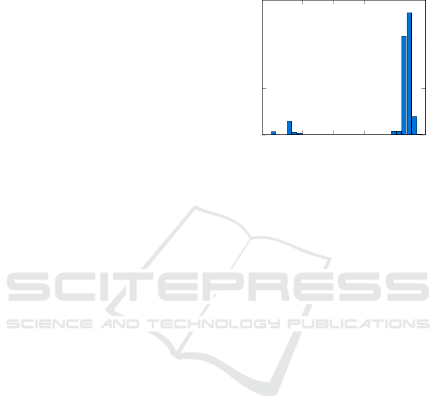
Figure 3: Histogram over the distribution of AKM-distances
between any two UNSPSC labels for τ = 3.
assigned a useful UNSPSC version 7.0401 label. UN-
SPSC is a 4-level hierarchical taxonomy, consisting
of the levels Segment, Class, Family, and Commodity,
mentioned in order of increasing specificity. For sim-
plicity, we will refer to these levels as level 1, level 2,
level 3, and level 4, respectively. Not all datapoints
contain a label at the lowest hierarchy level (level 4).
The distribution of labels among the 4 levels is roughly
as follows: at least on level 1:
100 %
, at least on level
2:
96 %
, at least on level 3:
83 %
, at least on level 4:
60 %
. We split the dataset into a 70/30 training and
test set, and then randomly shuffle each. Datapoints
from the test set have been removed if their label is not
present in the training set, resulting in a train and test
set split of
522,000
and
199,663
datapoints, respec-
tively, which we use for all further experiments.
Even though UNSPSC version 7.0401 contains
20,739
unique labels (including non-leaves), the
dataset includes only 3400 unique labels.
Figure 3 shows a histogram over
d
AKM
(y
i
, y
j
)
dis-
tances for all pairs of labels in the dataset. There are
a total of
50
buckets each distance can fall into. In-
creasing
τ
simply narrows the interval of the distances,
which is expected, due to
τ
appearing in the denomina-
tor in the definition of the AKM distance. This figure
shows that the distances between labels are grouped
into two groups. A path between two labels that passes
through the root incurs an AKM distance of at least
0.73
, independently of
τ
as level 1 contains
55
labels.
This means that label pairs in the smaller, leftmost
group share an ancestor different from the root. Those
in the rightmost, larger group, have a path that crosses
through the root. For
τ = 3
the mean AKM distance
for non-root crossing paths is
0.129
and
0.905
for root
crossing paths.
ICPRAM 2017 - 6th International Conference on Pattern Recognition Applications and Methods
506
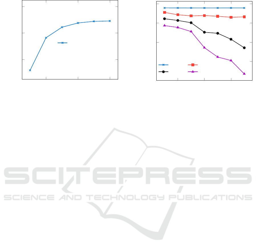
20 40 60
80
90
100
Top k % highest scoring features
Accuracy (%)
Logistic regression
Figure 4: Accuracy across feature percentages.
6.2 Results on UNSPSC Dataset
In this section, we formulate and discuss results from
experiments, on the UNSPSC-labeled invoice lines
dataset.
6.2.1 Choosing Features
We use a univariate feature selection method as de-
scribed in (Chen and Lin, 2006) to test the discrim-
inative power of different subsets of features. The
method calculates an F-score for each feature and, by
choosing the top
k
scoring features (those with high-
est F-values), a feature set is constructed from which a
predictive model is built. Figure 4 shows the accuracy
achieved on different feature sets using a standard mul-
ticlass logistic regression classifier on the test set. All
logistic regression classifiers used in this paper have
been made with the scikit-learn package (Pedregosa
et al., 2011).
It is evident that greater accuracies are achieved
with more features. However, it does not seem like the
accuracy will improve much beyond the top
40 %
fea-
tures. Therefore, as a trade-off between high accuracy
and time spent running tests, we use the top
40 %
of
features for further experiments.
6.2.2 τ Test
The
τ
value used in the definition of the AKM dis-
tance impacts to which extent higher level errors are
considered more costly than lower level errors. We
define the term level
k
matches to be the number of
datapoints that are correctly predicted at the
k
’th level,
out of the total number of datapoints that have a label
at the
k
’th level or below in the hierarchy. For exam-
ple, if a classifier predicts the label correct at the 2nd
level for
4500
out of
10,000
samples, the amount of
2 4 6
70
80
90
100
τ
Matches (%)
Level 1 Level 2
Level 3 Level 4
Figure 5: Level matches of AKM-EC in relation to τ .
level 2 matches is
4500/(10,000 · 0.96) = 43.2 %
,
since only
96 %
of the dataset has a label at the 2nd
or below. Figure 5 uses this measure to show that a
larger value of
τ
does in fact decrease the prediction
accuracy at lower levels, but slightly increases accu-
racy at the highest level. This is expected, as a higher
values of
τ
lowers the importance of accuracy at lower
levels.
6.2.3 Proof of Concept
The embedding classifiers are constructed to minimize
their respective distances between predicted and actual
labels in the dataset. Figure 6 compares the logistic
regression classifier to AKM-EC and EB-EC, accord-
ing to their respective distance measures. The figure
shows that they are very similar, and this is due to the
fact that logistic regression have an accuracy of
93.8 %
as shown in Figure 4, compared to
88.6 %
for AKM-
EC with dimension
150
. The high accuracy of logistic
regression results in a low average AKM distance, as
a correct prediction yields a distance of 0.
To compare how the classifiers deviate on errors
the misclassifications are isolated and evaluated as the
hierarchical properties proposed in Section 4.2.2 aims
to avoid root crossing paths. Figure 7 plots the aver-
age AKM and EB distances for each classifier across
dimensions on misclassified datapoints only. In this
figure, we see that AKM-EC minimizes the average
AKM distance, and the EB-EC minimizes the aver-
age EB distance, as expected. Notice how the EB and
AKM distances follow a similar pattern. This is also
expected, as the distances are similar see 4. AKM-
EC and EB-EC have lower distances than logistic re-
gression, because they optimize for their hierarchical
distance measures. Since logistic regression receive a
loss of 1 on misclassifications, we see that it perform
worse on each distance measure.
A Hierarchical Tree Distance Measure for Classification
507
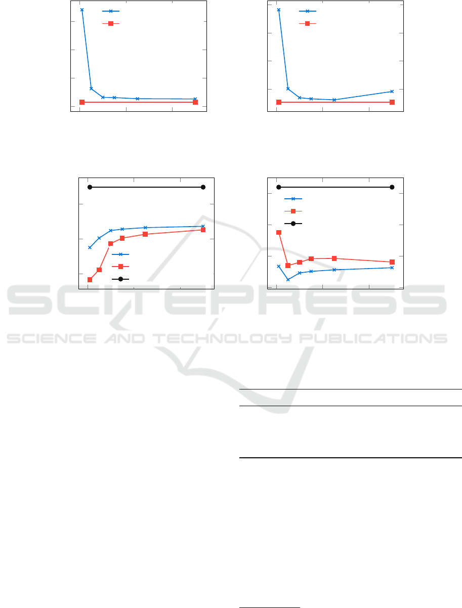
0 200 400
2
3
4
5
·10
−2
Dimensions
Average AKM distance
AKM-EC
Logistic regression
(a) Average AKM distance comparison for
τ = 3
.
0 200 400
0.3
0.4
0.5
0.6
Dimensions
Average EB distance
EB-EC
Logistic regression
(b) Average EB distance comparison.
Figure 6: Average AKM and EB distances for four different classifiers on the test dataset.
0 200 400
0.1
0.2
0.3
Dimensions
Average AKM distance
EB-EC
AKM-EC
Logistic regression
(a) Average AKM distances for τ = 3.
0 200 400
2.5
3
3.5
4
Dimensions
Averge EB distance
EB-EC
AKM-EC
Logistic regression
(b) Average EB distances across classifiers.
Figure 7: Average AKM and EB distances of embedding classifiers on the test dataset for misclassified samples.
For misclassifications, the average AKM distance
between the predicted and correct class for the AKM-
EC classifier is
0.213
, while the average AKM dis-
tance for logistic regression is
0.348
. In order to better
understand the meaning of these numbers, we calcu-
late the percent of non-root crossing paths during miss
classifications, this is calculated using the mean AKM
distance of non-root crossing paths and root crossing
paths from 3. For AKM-EC, this is
89 %
, meaning
only
11 %
of misclassifications have a path from the
predicted class to the actual class that crosses the root
node in the hierarchy. For logistic regression this is
72 %
, meaning
28 %
of misclassifications have a path
through the root node. This test shows the AKM-EC
comes with a trade-off between accuracy and lower
hierarchical distances on misclassifications.
6.3 Verification
In order to verify the properties of the AKM distance
measure, we compare the AKM-EC to the logistic re-
gression classifier and the EB-EC, on the
20
News-
groups dataset (20News, 2008). The AKM-EC and
Table 1: Classifier comparison on the Twenty Newsgroups
dataset between the AKM-EC and logistic regression classi-
fiers.
Metric AKM-EC Log. reg. EB-EC
Avg. AKM 0.219 0.24 0.203
AKM on miss 0.72 0.88 0.84
% correct 70 % 73 % 75 %
% root-crossing
2
49 % 62 % 58 %
the EB-EC are trained using 20 dimensions and
τ = 3
for AKM-EC. The average AKM distance of a root
crossing path using
τ = 3
for this dataset is
1.33
and
0.15
for a non-root crossing path these numbers are
used to calculated the
%
root crossing on misclassified
samples, which we aim to minimize with the AKM-
EC. The dataset contains
11,314
datapoints for train-
ing and
7532
datapoints for testing, organized into 20
classes. All the labels are at leaf nodes and the depth
of the hierarchy is 3.
Table 1 clearly shows that AKM-EC out performs
2
Calculated based on misclassified samples
ICPRAM 2017 - 6th International Conference on Pattern Recognition Applications and Methods
508

both logistic regression and the EB-EC when it comes
to minimizing the number of root crossing paths on
misclassification. The fact that the EB-EC have a
lower average AKM distance then AKM-EC is do to
it having a higher overall accuracy than the AKM-EC.
7 FUTURE WORK
In this section, we consider topics that could be ad-
dressed in future work.
Implementing a weighted algorithm when embed-
ding the
C
matrix could possibly improve the accu-
racy of the embedding classifiers. This is due to the
fact that, currently, label embeddings are independent
of how many datapoints of that label exist, possibly
resulting in labels with few samples causing noise.
Since the embedding classifier uses many linear re-
gressors, weighting the importance of each regressor’s
output in relation to its loss could possibly benefit clas-
sification.
There are also different ways of formulating a dis-
tance measure such that they are vastly different than
the AKM and EB measures, which take into account
properties of other hierarchies. It would be interesting
to evaluate how well the embedding classifier manages
to embed these distance measures.
One could consider expanding the 4-level UN-
SPSC tree to five or more levels.
8 CONCLUSION
We have introduced a novel hierarchical distance mea-
sure that aims to minimize the number of root crossing
paths. This measure fulfills the intuitive properties for
the UNSPSC product and service taxonomy. To take
advantage of this distance measure, we use an em-
bedding classifier, that embeds matrices representing
hierarchical distances to a lower-dimensional space.
In this space, datapoints are mapped to an embedded
class, and predictions are made. This classifier can be
combined with other distance measures. The results
presented in Section 6.2.3 and Section 6.3 shows that
using this distance measure lowers the number of root
crossing paths, at the cost of a slightly lower accuracy
when compared to logistic regression.
REFERENCES
20News (2008). 20 newsgroups. http://qwone.com/
∼
jason/
20Newsgroups/. Accessed: 2016-12-13.
Bishop, C. M. (2006). Pattern Recognition and Machine
Learning. Springer.
Chen, Y.-W. and Lin, C.-J. (2006). Feature Extrac-
tion: Foundations and Applications, chapter Combin-
ing SVMs with Various Feature Selection Strategies,
pages 315 – 324. Springer Berlin Heidelberg, Berlin,
Heidelberg.
Dumais, S. and Chen, H. (2000). Hierarchical classification
of web content. In Proceedings of the 23rd annual
international ACM SIGIR conference on Research and
development in information retrieval, pages 256 – 263.
ACM.
Labrou, Y. and Finin, T. (1999). Yahoo! as an ontology:
using yahoo! categories to describe documents. In
Proceedings of the eighth international conference on
Information and knowledge management, pages 180 –
187. ACM.
Pedregosa, F., Varoquaux, G., Gramfort, A., Michel, V.,
Thirion, B., Grisel, O., Blondel, M., Prettenhofer, P.,
Weiss, R., Dubourg, V., Vanderplas, J., Passos, A.,
Cournapeau, D., Brucher, M., Perrot, M., and Duch-
esnay, E. (2011). Scikit-learn: Machine learning
in Python. Journal of Machine Learning Research,
12:2825–2830.
Programme, U. N. D. (2016). United nations standard
products and services code homepage.
Silla, Carlos N., J. and Freitas, A. A. (2011). A survey of
hierarchical classification across different application
domains. Data Mining and Knowledge Discovery,
22(1 – 2):31 – 72.
Wang, K., Zhou, S., and Liew, S. C. (1999). Building
hierarchical classifiers using class proximity. In Pro-
ceedings of the 25th International Conference on Very
Large Data Bases, pages 363–374, San Francisco, CA,
USA. Morgan Kaufmann Publishers Inc.
Weinberger, K. Q. and Chapelle, O. (2009). Large margin
taxonomy embedding for document categorization. In
Koller, D., Schuurmans, D., Bengio, Y., and Bottou, L.,
editors, Advances in Neural Information Processing
Systems 21, pages 1737–1744. Curran Associates, Inc.
A Hierarchical Tree Distance Measure for Classification
509
