
Iterative Adaptive Sparse Sampling Method for Magnetic Resonance
Imaging
Giuseppe Placidi
1
, Luigi Cinque
2
, Andrea Petracca
1
, Matteo Polsinelli
1
and Matteo Spezialetti
1
1
A
2
VILab, Department of Life, Health & Environmental Sciences, University of L’Aquila, Via Vetoio, L’Aquila, Italy
2
Department of Computer Science, Sapienza University, Via Salaria, Rome, Italy
giuseppe.placidi@univaq.it, cinque@di.uniroma1.it, andrea.petracca@graduate.univaq.it,
matteo.polsinelli@student.univaq.it, matteo.spezialetti@graduate.univaq.it
Keywords:
Adaptive Acquisition Method, Sparse Sampling, Compressed Sensing, Undersampling, Sparsity, Reconstruc-
tion, Radial Directions, Projections, Non-linear Reconstruction.
Abstract:
Magnetic Resonance Imaging (MRI) represents a major imaging modality for its low invasiveness and for its
property to be used in real-time and functional applications. The acquisition of radial directions is often used
but a complete examination always requires long acquisition times. The only way to reduce acquisition time is
undersampling. We present an iterative adaptive acquisition method (AAM) for radial sampling/reconstruction
MRI that uses the information collected during the sequential acquisition process on the inherent structure of
the underlying image for calculating the following most informative directions. A full description of AAM is
furnished and some experimental results are reported; a comparison between AAM and weighted compressed
sensing (CS) strategy is performed on numerical data. The results demonstrate that AAM converges faster
than CS and that it has a good termination criterion for the acquisition process.
1 INTRODUCTION
Magnetic Resonance Imaging (MRI) is a major non-
invasive imaging modality, due to its ability to provide
anatomical details and information on physiological
status and pathologies. The reconstruction of a sin-
gle image usually involves the acquisition of a series
of trajectories. The measurement of a trajectory is a
sampling process of a function evolving with time in a
domain referred to as k-space. Raw data are then used
to reconstruct the images (O’Sullivan, 1985; Jackson
et al., 1991). The most popular k-space trajectories
are straight lines on a Cartesian grid, in which each
k-space line corresponds to the frequency encoding
readout at each value of the phase encoding gradient
(Spin Warp Imaging, (Edelstein et al., 1980)). The
lines in the grid are parallel and equally separated.
Although the acquisition of Cartesian trajectories al-
lows easier image reconstruction, recent advances in
MRI hardware allow other acquisition patterns, such
as spirals (Meyer, 1998), radial trajectories (Projec-
tion Reconstruction, PR (Lauterbur, 1973)) and other
curve trajectories (Placidi, 2010). PR, in particular,
is fundamental for real time and functional MRI ap-
plications because it reduces the effects due to mo-
tion and improves the signal to noise ratio (SNR) in
the reconstructed image (the center of k-space is over-
sampled). In these applications, the gain in the recon-
structed images, both in artifacts reduction and in im-
provement of functional information, is proportional
to the time saved during acquisition.
The acquisition process for MRI can be defined by
the following linear system:
y = Ax+ z (1)
where y are the linear measurements of a h dimen-
sional vector in the k-space, A is an hxM matrix of h
directions, x is the unknown MxM image and z is a
Gaussian noise added to the measurements.
A fundamental limitation of MRI is the linear rela-
tion between the number of acquired trajectories and
net scan time (Eq. 1): minutes are often required to
collect a complete data set. Such duration can be too
high when dynamic processes have to be observed at
high temporal resolution, as for example in functional
studies (Bernstein et al., 2004). Moreover, the im-
age quality can be lowered by the presence of move-
ment artifacts intrinsic to the observed dynamic pro-
cess. The acquisition time for each trajectory is lim-
ited by the slow natural relaxation times which are be-
yond the control of the acquisition sequence and have
to be waited. The only way to speed up acquisition is
510
Placidi, G., Cinque, L., Petracca, A., Polsinelli, M. and Spezialetti, M.
Iterative Adaptive Sparse Sampling Method for Magnetic Resonance Imaging.
DOI: 10.5220/0006199105100518
In Proceedings of the 6th International Conference on Pattern Recognition Applications and Methods (ICPRAM 2017), pages 510-518
ISBN: 978-989-758-222-6
Copyright
c
2017 by SCITEPRESS – Science and Technology Publications, Lda. All rights reserved

to reduce the number of trajectories, that is by using
undersampling. Undersampling is the violation of the
Nyquists criterion where images are reconstructed by
using a smaller number of samples than what is the-
oretically required to obtain a fully sampled image.
One of these methods (Placidi et al., 2000) presented a
k-space adaptive acquisition technique that calculated
the information content of the collected projections to
drive the measurements of the following projections.
Modified Fourier reconstruction algorithm, including
an interpolation method (Placidi et al., 1998; Placidi
and Sotgiu, 2004), were used to reconstruct the im-
age from the resulting sparse set of projections. The
same algorithm was also used in the field of image
compressing (Placidi, 2009a). Other authors (Can-
des et al., 2006; Donoho, 2006) presented the the-
ory of Compressed Sensing (CS) and the details of its
implementation for rapid MRI (Lustig et al., 2007).
CS allows accurate reconstruction of images with far
fewer measurements than traditional methods, when
two requirements are met: sparsity and incoherence.
Sparsity means that the image information can be rep-
resented, in some domain, using a small number of
coefficients without compromising the image quality.
Incoherence implies that the energy of objects in the
sparse domain is spread out in the measurement do-
main. CS in MRI typically uses wavelet transform
to promote sparsity and random k-space sampling to
ensure incoherence. If sparsity and incoherence are
satisfied, an image can be recovered to high accuracy,
even if k-space is significantly undersampled,by solv-
ing the following convex optimization:
min
x
kΨxk
1
: ky− Φxk ≤ ε, (2)
Here, y are the acquired k-space samples in the
Fourier Space, Φ is the Fourier transform and Ψ is
a transform where the image is sparse (wavelet trans-
form is used therein), and ε is a threshold level that
bounds the noise.
Most of the CS applications used the l
1
-norm min-
imization as reconstruction method. Reconstruction
can also be improved by increasing samples in the
central part of the k-space, because low frequency
terms contain more energy than high frequency terms,
as demonstrated in weighed CS (Wang and Arce,
2010; Magnusson et al., 2010). In (Arias-Castro et al.,
2013) the authors discussed the limits of any adap-
tive sensing technique with respect to the classical
CS scheme in the sense that, if we have a number
of measurements sufficiently high (this ”sufficiently
high” number is very hard to estimate when nothing
is known about the underlying image), the error ob-
tained by classical CS acquisition/reconstruction pro-
cess is almost equivalent to that obtained by a ”smart”
adaptive acquisition/reconstruction method. Though
this is right, it has been shown elsewhere (Placidi
et al., 2000; Placidi et al., 2014; Placidi, 2014; Cian-
carella et al., 2012; Placidi, 2009b) that it may be
possible to reduce the minimum number of necessary
projections (Brooks and Di Chiro, 1976), if infor-
mation about sample internal symmetries and shape
can be collected during acquisition. These methods,
though very effective in reducing acquisition time
while obtaining high quality images, are not optimal
in the estimation of the image sparsity value and re-
quire highly specialized software (dedicated hardware
is also recommended). We present a simple iterative
adaptive sparse acquisition strategy for radial (PR)
sampling/reconstruction MRI that uses the inherent
structure of the underlying image for obtaining an ef-
ficient adaptive acquisition method (AAM). In what
follows, a full description of AAM is furnished and
some experimental results are reported; a comparison
between the proposed technique and weighted CS is
performed on numerical data. The main advantages
of AAM with respect to weighted CS are that its esti-
mation error could converge faster than CS and that
AAM detailed an accurate estimate of the sparsity
value of the underlying image, that is a good termi-
nation criterion for the acquisition process.
2 MATERIALS AND METHODS
The proposed AAM is a variant of a deterministic
acquisition method (ADM) or CS strategy, with the
advantage of eliminating the blind phase during the
acquisition process by using a choice mechanism to
select the acquisition trajectories that are most ”infor-
mative”, basing on the shape of the underlying image
(Figure 1).
AAM is an iterative process that analyses the data
acquired during the sequential acquisition phase in or-
der to obtain useful information regarding the follow-
ing most ”informative” directions to be explored: the
process is adaptive in the sense that it adapts the fol-
lowing directions to the shape of the object under in-
vestigation. The information regarding the shape of
the object are collected starting by an initial subset of
the possible directions and used to reconstruct an ap-
proximation of the object. The following refinements
are obtained by integrating the initial set with other
directions collected where highest is the information
content.
Iterative Adaptive Sparse Sampling Method for Magnetic Resonance Imaging
511
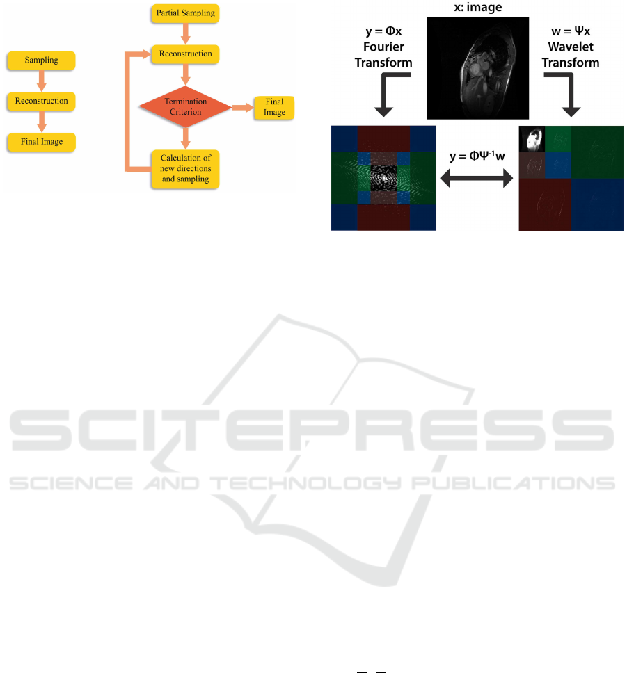
Figure 1: AAM (right) is different with respect to ADM or
CS (left) because ADM and CS use a pre-determined set of
regular (ADM) or random directions (CS) while AAM uses
the information collected during the previous acquisition
steps for the calculation of the following directions where
the information content is maximum. Moreover AAM is
adaptive with respect to the shape of the unknown image
and it contains a termination criterion to stop acquisition
when the resulting image has reached the maximum qual-
ity.
2.1 Relationship between an Image and
Its Wavelet e Fourier Domains
The use of wavelets in MRI is not new: examples can
be found in (Sung and Hargreaves, 2013; Chen and
Huang, 2012).
Since data in MRI are collected in the k-space (the
Fourier domain), the relationship between the Fourier
and Wavelet domains of a give image, well described
in (Sung and Hargreaves, 2013; Gonzalez and Woods,
2007), can be used. This relationship allows to sepa-
rate the k-space in different regions corresponding to
different Wavelet subbands.
In fact, given an image, its Fourier and Wavelet
transforms are related as shown in Figure 2. The ap-
proximation image in the wavelet domain (right part
of the figure, higher left square) has a Fourier trans-
form that corresponds to the central window of the
Fourier coefficients of the complete image (left part of
the figure, central square). Analogously, the wavelet
coefficients of the details (in red, blue and brown
coloured regions) have their correspondence in the re-
gions indicated on the left with the same combination
of colors.
Figure 2 directly correlates the coloured subbands
to the regions with the same colors in the k-space,
each wavelet level corresponding to a specific Fourier
frame.
The previous relationship can be used to reformu-
late the reconstruction problem of Eq. 2 as follows
(see Figure 2 for convenience):
min
w
kwk
1
: ky− ΦΨ
−1
wk ≤ ε. (3)
Figure 2: Relationship between image domains: x=image
space, y=Fourier space, w=Wavelet space.
In this case, the matrix A in Eq. 1 is A = ΦΨ
−1
Ψ = Φ.
The problem can be interpreted as to find x such that x
is sparse in the Wavelet domain (Ψx = w) and that its
representation in the Fourier domain (ΦΨ
−1
w = Φx)
is very close to what has been acquired (Φx = y).
A is the matrix connecting the two domains: one,
the Fourier domain, in which data are collected and
the other, the Wavelet domain, necessary to promote
sparsity.
2.1.1 Upsampling in the Wavelet Domain
The previous relationship can be used for reconstruc-
tion purposes (Sung and Hargreaves, 2013) but, more
importantly for our problem, also for acquisition pur-
poses, that is to drive the acquisition process towards
the most informative regions of the image wavelet
space and, hence, of the Fourier space.
It is important to note that in Figure 3 the central
region of the k-space represents an approximation of
the complete image.
For example, by considering the image of size
MxM (M=256) in Figure 3, if we select a square
of Fourier coefficients around the k-space center of
size
M
2
x
M
2
and use these data to reconstruct the im-
age (through FFT), the resulting image will have half
resolution of the original image but the shape of the
image is still well recognizable. What has been lost
are the horizontal, vertical and diagonal details that
are described by the excluded high frequency coeffi-
cients (region external to the red square in Figure 3).
Since the selected approximation maintains most
of the features of the original image, it can be ar-
gued that there is a strict correlation between the com-
pletely sampled image and each of its approxima-
tions, to any level (the correlation is greater for levels
closer to the considered approximation).
ICPRAM 2017 - 6th International Conference on Pattern Recognition Applications and Methods
512
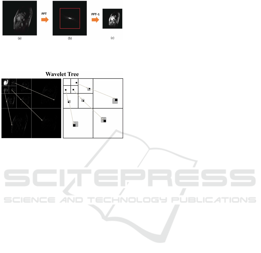
Figure 3: (a) Original 256x256 image; (b) k-space repre-
sentation with a selected central region of size 128x128; (c)
Reconstructed 128x128 image obtained by Fourier trans-
forming the selected k-space region.
Figure 4: Wavelet coefficients tree structure. In the left
panel, the wavelet transform of a real image is shown; in
the right panel, the corresponding scheme is reported by us-
ing an inverted color palette, for convenience.
Such correlation is codified in the wavelet domain
with a tree structure existing between the different
levels of each component (see Figure 4). If relevant
information are present on the root, it is highly prob-
able that relevant information are present also at the
details levels. This correlation can be used also in
the negative case: if relevant information are absent
on the root, it is highly probable that they will be ab-
sent also at the details levels. This property can be
used to compress the image: set 0 the details deriving
from an irrelevant root coefficient. This tree struc-
ture is defined quadtree (Sung and Hargreaves, 2013).
A quadtree is a tree of positions in which, starting
from a root [i, j], its child are positioned at [2i,2j],
[2i+ 1, 2j], [2i,2j + 1], [2i+ 1,2j + 1].
By knowing the position of an irrelevant (respec-
tively, relevant) wavelet coefficient at a root of a
quadtree we can assume information regarding the
irrelevance of all its descendants in the tree (respec-
tively, we can define a further wavelet decomposition
of the current root image and, by using the correlation
between the new root and its child, it is possible to es-
timate the details at finer scales, that is to interpolate).
If we iterate this process, we can reach the original
image details, as described below.
2.2 The Proposed Method
AAM is an iterative method that uses the relationship
between the collected data in the k-space, the image
space and the wavelet space, as reported in the flow-
chart of Figure 5.
In this case, the wavelet space is used as a support
space for its good properties of multiresolution (it is
simple and effective to estimate image details starting
from its raw approximation, without producing alias-
ing) and locality (errors due to estimation are confined
around the point in which they were produced, not af-
fecting the whole image). In words (see Figures 5
and 6), AAM starts by considering a subset of equi-
spaced radial directions: for the given dataset, would
exist a reduced square support in the Fourier space for
which the resulting image is fully sampled (square n.1
in Figure 6). Then, for this supportthe image is recon-
structed. If the maximum image support is reached,
the process is terminated and the reconstructed image
is the final image. Otherwise, the wavelet transform
of the image is calculated and the horizontal, vertical
and diagonal details are estimated: the image is up-
sampled of a factor of 2 in the wavelet domain. Then,
the inverse wavelet transform is calculated and finally
the inverse Fourier transform of the resulting image
is performed. In this case, a Fourier support double
than the previous is obtained for the unknown image
(square n.2 in Figure 6). At this step, the mean power
spectrum is calculated for each circular segment (cir-
cular segments are comprised between circles n.1 and
n.2 and separated by contiguous radial directions in
Figure 6) and the vector E, containing the mean power
spectrum values, is ordered in descending order. As
long as max(E) > ε (ε is a power spectrum threshold
that will be defined below), repeat the measurement
of a new radial direction between the two directions
where max(E) is present, update the E values and re-
order them in a descending order. Return to the ”SET
DIM VALUE” point in Figure 5. It is important to
note that, during the intermediate steps, the newly col-
lected radial directions cover the whole image support
and not just the current reduced square.
2.2.1 Acquisition Parameters
The user-defined parameters are, in this case, two: the
number of equispaced radial directions to start the ac-
quisition process that, implicitly, depends on the size
of the k-space support of the first approximation im-
age (square n.1 in Figure 6); the ε valuecorresponding
to the noise level, the same used in the reconstruction
process (Eq. 2) as a termination parameter. Both these
parameters can be simply calculated. In fact, the first
approximation support is M/8 (the size of square n.1
Iterative Adaptive Sparse Sampling Method for Magnetic Resonance Imaging
513
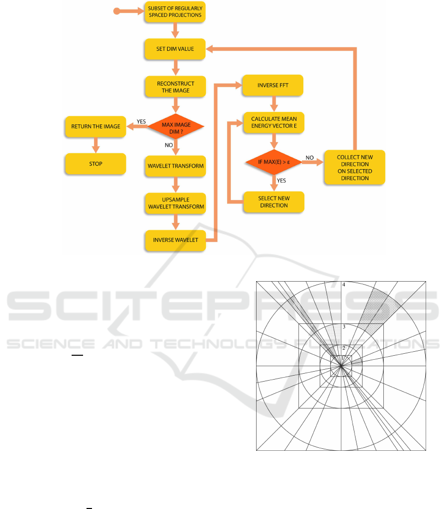
Figure 5: Flow-chart of the AAM.
in Figure 6), having considered M as a power of two
(intrinsic MRI resolution usually implies M = 256).
In this case, having supposed each radial direction is
sampled on M points (each with M/8 points on circle
n.1 in Figure 6), the number of equally spaced radial
directions m
0
to fill uniquely the circle n.1 in Figure
6 is about m
0
∼
=
πr
2
p
d
(the area of a circle calculated
as the number of pixels contained inside it divided by
the number of samples of each radial direction falling
inside the circle) where r = M/16 is the circle radius
in pixels and p
d
= M/8 is the number of points of
each radial direction falling inside the circle (Brooks
and Di Chiro, 1976; Placidi et al., 1995)). In our case,
having considered images where M = 256 and a first
approximation support of M/8 = 32, it follows that
r = 16, p
d
= 32 and m
0
= 26. The second parameter,
ε, represent the noise level, the mean power spectrum
level of the noise (Placidi et al., 2000):
ε =
1
s
s
∑
i=1
(R
2
i
+ I
2
i
), (4)
in which s is the number of samples of different ra-
dial directions falling outside the circle n.4, where just
noise is present because out the image support and R
i
and I
i
are the real and imaginary components of each
data sample, respectively. These data are collected
when the first set of radial directions is measured by
prolonging the measurement of each direction: the
time used does imply no wast of time because it uses
Figure 6: AAM operative example. The highlighted circular
segments represent those where higher is the mean power
and a new radial direction is collected.
the temporal interval necessary to recover the spin
magnetization (Placidi, 2012).
3 EXPERIMENTS
Simulations are performed on cardiac MRI com-
pletely sampled 4D data, from a dataset of 240 images
(image size 256x256 pixels, 65.536 samples) consist-
ing of 20 temporal frames (time=1,.. .,20) and 12 x-y
ICPRAM 2017 - 6th International Conference on Pattern Recognition Applications and Methods
514
slices along the z axis (depth=1,...,12).
To perform the tests, full acquisitions are simu-
lated through the Fourier transform of completely re-
constructed images. In this way the complete datasets
of the k-space samples are assumed. In order to sim-
ulate undersampled acquisitions, binary masks, con-
taining ”1” where the coefficients have to be col-
lected and ”0” where the coefficients have to be dis-
carded, are multiplied, point by point, with the com-
plete datasets.
This operation, though does not reflect precisely a
real experimentalprocess (phase errors, off-resonance
effects, thermal instability, etc., are not considered), is
useful for having a complete reference image that can
be used to estimate the performance AAM in terms of
Mean Square Error (MSE) with respect the fully sam-
pled. In this way, a wrong reconstruction can only be
due to a wrong sampling/reconstruction method and
not also to other experimental factors.
The images obtained with AAM are compared
with those of a weighted CS, in which a dou-
ble random acquisition along cartesian directions,
rows/columns, is performed by using a normalised
Gaussian weighted function with µ = 0 (0 indicates
that the mean value is in the k-space center) and σ = 1
(1 indicates a distance equal to 64 rows/columns from
the center): this weight is chosen to prefer the k-space
central area where the image power is higher with re-
spect to the peripheral zones.
The CS sampling/reconstruction process, being a
single step reconstruction, is performed by changing
the number of rows and columns (the number of rows
is equal to the number of columns). The dataset starts
from 7000 samples with increments of 5.000 samples,
until an almost completely sampled image is reached.
It is important to note that for each dataset the ac-
quisition process restarts from the beginning, without
increasing the dataset collected in the previous steps.
The starting value for the weighted CS (7.000
samples) is completely arbitrary and it is just used to
compare the CS results with the starting dataset used
for the AAM (that equals to 6656 samples, being the
result of 26 starting projections each containing 256
sampled). The sequence of AAM images are obtained
by adding, at each step of the algorithm, the new
directions adaptively selected: the dataset grows by
adding new directions to those previously collected.
The resulting image, both for the CS and for all
the steps of AAM, is obtained by using the l
1
-norm
minimization.
The tests are executed in MatLab R2015a
(http://www.mathworks.com) on a workstation
equipped with operating system Windows 7, a
processor Intel (R) Core (TM) I7-6700 (3.40 Ghz),
16 GB of RAM and an SSD drive.
Aim of the performed simulations is to show that
AAM is really able to identify/collect the most infor-
mative directions by comparing its results with CS,
used for reference. Moreover, it is also useful to ver-
ify the AAM stopping criterion and its good capa-
bility in estimating the sparsity value of the under-
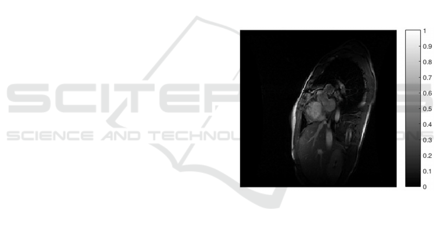
lying image. The tests have been conducted on the
whole dataset of 240 images but the results are shown
just for a single image, being the others very simi-
lar (the images have similar shape and support, espe-
cially those allowing to the same time instant). The
details of the tests, performed with the image z = 1
and time 3 (Figure 7), are reported in Figure 8 where
the MSE is calculated for each of the intermediate re-
constructions. Figure 9 and Figure 10 show the con-
servation of the image wavelet coefficients for an in-
termediate reconstruction both for AAM (intermedi-
ate reconstruction with 11520 collected samples) and
CS (17000 samples).
Figure 7: One of the test images: z=1, time=3.
In particular, it can be noted that for AAM most
of the wavelet coefficients correspond to those of
the original image (wrongly placed or missing coef-
ficients are very few, as indicated by the red zones in
Figure 9); on the contrary, for the CS image most of
the wavelet coefficients are wrongly placed (artifacts
are evident outside the image support in the wavelet
image) or lost (red zones in Figure 10).
This is also confirmed by corresponding MSE val-
ues (Figure 8): the MSE for the AAM intermediate
reconstruction is about one order of magnitude lower
than that of CS, though by using a lower number of
samples. From Figure 8, it is very interesting to note
that the MSE values for AAM is constantly descen-
dent while this does not occur for CS (the CS dataset,
being re-sampled, could encounter ”unfortunate” di-
rections); moreover, the MSE of AAM is constantly
Iterative Adaptive Sparse Sampling Method for Magnetic Resonance Imaging
515
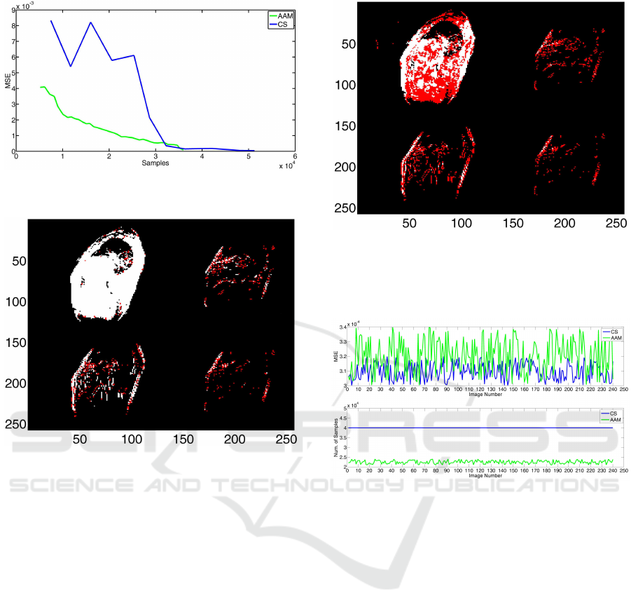
Figure 8: Calculated MSE for intermediate reconstructions
of AAM (green line) and for CS (blue line).
Figure 9: Wavelet correspondences between AAM interme-
diate reconstruction with 11520 samples and the fully sam-
pled image. White are the correctly placed coefficients. Red
are the missing or wrongly placed coefficients with respect
to the original image.
below that of CS (CS converges to that of AAM when
a high number of samples is used).
On the contrary, the termination criterion used for
AAM allows to stop the acquisition process when the
MSE becomes plateful (92 directions with 23552 co-
efficients were used). The calculated value is a good
approximation of the sparsity value of the original im-
age. In fact, by performingthe wavelet transformation
of the original image with a threshold on the noise
level, the calculated sparsity value is 18170. The same
MSE value is reached by CS at 32000, about 29%
more samples than those necessary for AAM. More-
over, CS requires to go over 32000 in order to reduce
the probability of a wrong reconstruction, since it has
no way to know in advance the sparsity of the under-
lying image. The results obtained for the whole image
dataset are summarized in Figure 11). As can be ob-
served: 1) the MSE values obtained with the AAM
method are very close to, in some cases also better
than, those obtained by CS, though the images are
obtained with less than 60% of the coefficients used
Figure 10: Wavelet correspondences between CS recon-
struction with 17000 samples and the fully sampled image.
White are the correctly placed coefficients. Red are the
missing or wrongly placed coefficients with respect to the
original image.
Figure 11: Calculated MSE (up) and final number of sam-
ples (down) used for AAM (green line) and CS (blue line)
reconstructions of each image composing the dataset. The
number of samples for CS is always 40000.
for CS; 2) for CS a fixed number of 40000 samples
are used since it does not use the sparsity of the im-
age; 3) the number of coefficients calculated by AAM
slightly oscillates around 22000, having the images
of the dataset very similar shape (heart moves and
changes but chest and lungs structures remain almost
unchanged).
4 CONCLUSIONS
We have presented an iterative adaptive acquisition
method for radial sampling/reconstruction in MRI
that uses the information on the inherent structure
of the underlying image collected during the sequen-
tial acquisition process for calculating the following
most informative directions. The method has been
described and some experimental results reported.
A comparison between the proposed method and a
ICPRAM 2017 - 6th International Conference on Pattern Recognition Applications and Methods
516

weighted compressed sensing strategy was performed
on a cardiac MRI examination composed by 240 im-
ages. The images were compared both visually and
through the MSE evaluation with respect to the com-
pletely sampled version of each image. The results
demonstrated that AAM converged faster than CS by
using just the necessary coefficients (about 55% of
those used by CS). Future research will be spent for
evaluating the performance of AAM with respect to
other adaptive acquisition schemes.
ACKNOWLEDGEMENTS
The Authors are grateful to Mrs Carmelita Marinelli
for technical assistance.
REFERENCES
Arias-Castro, E., Candes, E., and Davenport, M. (2013).
On the fundamental limits of adaptive sensing. IEEE
Transactions on Information Theory, 59(1):472–481.
Bernstein, M., King, K., and Zhou, X. (2004). Handbook of
MRI Pulse Sequences. Elsevier Academic Press.
Brooks, R. and Di Chiro, G. (1976). Principles of com-
puter assisted tomography (cat) in radiographic and
radioisotopic imaging. Physics in Medicine and Biol-
ogy, 21(5):689–732.
Candes, E., Romberg, J., and Tao, T. (2006). Robust
uncertainty principles: exact signal reconstruction
from highly incomplete frequency information. IEEE
Transactions on Information Theory, 52(2):489–509.
Chen, C. and Huang, J. (2012). Compressive sensing mri
with wavelet tree sparsity. In Advances in Neural In-
formation Processing Systems, pages 1124–1132.
Ciancarella, L., Avola, D., Marcucci, E., and Placidi, G.
(2012). A hibrid sampling strategy for sparse mag-
netic resonance imaging. In Computational Mod-
elling of Objects Represented in Images. Fundamen-
tals, Methods and Applications, pages 285–289, Boca
Raton – USA. CRC Press, Taylor & Francis Group.
Donoho, D. (2006). Compressed sensing. IEEE Transac-
tions On Information Theory, 52(4):1289–1306.
Edelstein, W., Hutchison, J., Johnson, G., and Redpath, T.
(1980). Spin warp nmr imaging and applications to
human whole-body imaging. Physics in Medicine and
Biology, 25(4):751–756.
Gonzalez, R. and Woods, R. (2007). Digital Image Process-
ing (3rd Edition). Pearson.
Jackson, J., Meyer, C., Nishimura, D., and Macovski, A.
(1991). Selection of a convolution function for fourier
inversion using gridding [computerised tomography
application]. IEEE Transactions on Medical Imaging,
10(3):473–478.
Lauterbur, P. (1973). Image formation by induced local in-
teractions: examples employing nuclear magnetic res-
onance. Nature, 242(5394):190–191.
Lustig, M., Donoho, D., and Pauly, J. (2007). Sparse
mri: The application of compressed sensing for
rapid mr imaging. Magnetic Resonance in Medicine,
58(6):1182–1195.
Magnusson, M., Leinhard, O., Brynolfsson, P., Thyr, P., and
Lundberg, P. (2010). 3d magnetic resonance imag-
ing of the human brain - novel radial sampling, fil-
tering and reconstruction. In 12th IASTED Interna-
tional Conference on Signal and Image Processing
(SIP 2010). ACTA Press.
Meyer, C. (1998). Spiral echo-planar imaging, pages 633–
658. Springer Berlin Heidelberg.
O’Sullivan, J. (1985). A fast sinc function gridding algo-
rithm for fourier inversion in computer tomography.
IEEE Transactions on Medical Imaging, 4(4):200–
207.
Placidi, G. (2009a). Adaptive compression algorithm from
projections: Application on medical greyscale im-
ages. Computers in biology and medicine, 39:993–
999.
Placidi, G. (2009b). Constrained reconstruction for sparse
magnetic resonance imaging. In World Congress
on Medical Physics and Biomedical Engineering,
September 7 - 12, 2009, Munich, Germany, vol-
ume 25/4, pages 89–92, Berlin Heidelberg – DEU.
Springer.
Placidi, G. (2010). Circular acquisition to define the mini-
mum set of projections for optimal mri reconstruction.
Lecture notes in computer science, 6026:254–262.
Placidi, G. (2012). MRI: essentials for innovative technolo-
gies. CRC Press, Taylor & Francis Group, Boca Raton
– USA.
Placidi, G. (2014). Recent advances in acquisi-
tion/reconstruction algorithms for undersampled mag-
netic resonance imaging. Journal of biomedical engi-
neering and medical imaging, 1:59–78.
Placidi, G., Alecci, M., Colacicchi, S., and Sotgiu, A.
(1998). Fourier reconstruction as a valid alternative to
filtered back projection in iterative applications: Im-
plementation of fourier spectral spatial epr imaging.
Journal of Magnetic Resonance, 134(2):280–286.
Placidi, G., Alecci, M., and Sotgiu, A. (1995). Theory of
adaptive acquisition method for image reconstruction
from projections and application to epr imaging. Jour-
nal of magnetic resonance. Series A, 108:50–57.
Placidi, G., Alecci, M., and Sotgiu, A. (2000). Omega-
space adaptive acquisition technique for magnetic res-
onance imaging from projections. Journal of Mag-
netic Resonance, 143(1):197–207.
Placidi, G., Avola, D., Cinque, L., Macchiarelli, G., Pe-
tracca, A., and Spezialetti, M. (2014). Adaptive sam-
pling and non linear reconstruction for cardiac mag-
netic resonance imaging. In Computational Modeling
of Objects Presented in Images Fundamentals, Meth-
ods, and Applications, volume 8641, pages 24–35.
Placidi, G. and Sotgiu, A. (2004). A novel restoration
algorithm for reduction of undersampling artefacts
Iterative Adaptive Sparse Sampling Method for Magnetic Resonance Imaging
517

from magnetic resonance images. Magnetic reso-
nance imaging, 22:1279–1287.
Sung, K. and Hargreaves, B. (2013). High-frequency sub-
band compressed sensing mri using quadruplet sam-
pling. Magnetic Resonance in Medicine, 70(5):1306–
1318.
Wang, Z. and Arce, G. (2010). Variable density compressed
image sampling. IEEE Transactions on Image Pro-
cessing, 19(1):264–270.
ICPRAM 2017 - 6th International Conference on Pattern Recognition Applications and Methods
518
