Studying Stability of Different Convolutional Neural Networks Against
Additive Noise
Hamed H. Aghdam, Elnaz J. Heravi and Domenec Puig
Computer Engineering and Mathematics Department, Rovira i Virgili University, Tarragona, Spain
Keywords:
Adversarial Examples, Convolutional Neural Networks, Fourier Transform.
Abstract:
Understanding internal process of ConvNets is commonly done using visualization techniques. However, these
techniques do not usually provide a tool for estimating stability of a ConvNet against noise. In this paper, we
show how to analyze a ConvNet in the frequency domain. Using the frequency domain analysis, we show the
reason that a ConvNet might be sensitive to a very low magnitude additive noise. Our experiments on a few
ConvNets trained on different datasets reveals that convolution kernels of a trained ConvNet usually pass most
of the frequencies and they are not able to effectively eliminate the effect of high frequencies.They also show
that a convolution kernel with more concentrated frequency response is more stable against noise. Finally, we
illustrate that augmenting a dataset with noisy images can compress the frequency response of convolution
kernels.
1 INTRODUCTION
In the task of object recognition, the input of a Convo-
lutional Neural Networks (ConvNets) is usually a 3-
channel image. Consequently, dimensions of the fil-
ters in the first convolution layer could be w
1
×h
1
×3.
Assuming that the first layer consists of K filters, the
input to the second convolution layer might be a K-
channel image where each channel is called a fea-
ture map. Also, the dimensions of the filters might
be w
2
×h
2
×K. Since convolution filters are the main
building block of ConvNets it is crucial to understand
what happens when the input image is convolved us-
ing these filters. Also, we may be able to decipher
the function of each layer in a ConvNet by analyzing
each filter separately. However, interpreting 3D filters
is not trivial in spatial domain. Specially, in the case
of ConvNets, the third dimension of the filters is usu-
ally high since they depend on the number of the input
channels which makes them harder to be understood.
There is a large body of work on understanding the
internal process of ConvNets through visualization of
hidden units. (Zeiler and Fergus, 2013) visualize the
hidden units using Deconvolutional Networks. To be
more specific, they reconstruct the images which have
highly activated each unit. By this way, we can as-
sess how each unit see the world and which parts of
objects activate each neuron more. (Simonyan et al.,
2013) find a L
2
-regularized image for each class by
maximizing the class specific score. They also com-
pute a class saliency map for the input image.
(Girshick et al., 2014) keep record of activations
for a specific unit by entering many images to Con-
vNet and calculating their activations on the unit.
Then, the images are sorted according to their acti-
vation on this particular unit and illustrated. Taking
into account the fact that each unit in top layers has a
corresponding receptive field on the image, it is pos-
sible to see which parts are important for each unit.
(Mahendran and Vedaldi, 2014) invert the d-
dimensional representation of an image computed by
function Θ : R
H×W ×C
−→ R
d
. This approach tells
us that to which extend it is possible to reconstruct
the image using the representation function Θ. By
applying this method on each layer of the network
we can understand which information is preserved by
each layer. Similarly, (Dosovitskiy and Brox, 2015)
reconstructed the image by minimizing the squared
Euclidean between the downsampled image and re-
constructed image. Recently, (Nguyen et al., 2015)
developed an evolutionary algorithm for generating
images that do not look like to any of objects in the
database but are classified with high score by Con-
vNet into one of object classes. Even though the visu-
alization approaches help us to better understand the
internal process of ConvNets, they do not provide a
tool for assessing the stability of a ConvNet against
noise. To address this problem, (Szegedy et al., 2013)
proposed a method for finding a L
2
regularized ad-
ditive noise which minimizes the score of a specific
362
Aghdam H., J. Heravi E. and Puig D.
Studying Stability of Different Convolutional Neural Networks Against Additive Noise.
DOI: 10.5220/0006200003620369
In Proceedings of the 12th International Joint Conference on Computer Vision, Imaging and Computer Graphics Theory and Applications (VISIGRAPP 2017), pages 362-369
ISBN: 978-989-758-226-4
Copyright
c
 2017 by SCITEPRESS – Science and Technology Publications, Lda. All rights reserved

class.
Contribution: In practice, it is necessary to ex-
amine how stable are ConvNets when the input image
is noisy. This is empirically achievable by evaluating
ConvNets using a contaminated test set. Another way
is to analyze filters in each layer in domains rather
than the spatial domain. In this paper, we show how to
analyze the filters of different layers in the frequency
domain (Section 2). Then, we empirically assess var-
ious ConvNet architectures on different object recog-
nition datasets (Section 3). The experiments try to
compare various choices for the loss function, acti-
vations and the input size. Moreover, they illustrate
that training a ConvNet using a noisy training set may
increase the stability of the network. Above all, we
analyze the ConvNets in the frequency domain to find
out why all ConvNets are sensitive to small changes
in the input.
2 ANALYSIS IN THE
FREQUENCY DOMAIN
Fourier transform decomposes a N-dimensional sig-
nal into N-dimensional sin and cos functions with var-
ious frequencies. The strength of each frequency is
indicated by the magnitude of the sin and cos func-
tions for that particular frequency. Mathematically,
the Fourier transform of a 3-dimensional signal is de-
fined as follows:
F (E
1
, E
2
, E
3
) =
Z
∞
−∞
Z
∞
−∞
Z
∞
−∞
Hdx
1
dx
2
dx
3
H = e
−2πi(x
1
E
1
+x
2
E
2
+x
3
E
3
)
f (x
1
, x
2
, x
3
)
(1)
In this equation, E
i
is the frequency along i
th
axis
and f is a 3-D signal. In the case of ConvNets, f
could be a 3D convolution kernel or a 3D feature map.
F (E
1
, E
2
, E
3
) is a complex number indicating the
magnitude and phase of frequency triple (E
1
, E
2
, E
3
)
in signal f . Frequency response of a filter/feature map
can be obtained by computing (1) on every spatial lo-
cation on the filter/feature map. Visualizing the fre-
quency response of a filter shows the frequencies that
are blocked and passed by the filter. For example,
Sobel filter is the common choice for calculating the
first derivative of an image compared with other well-
known 3 × 3 edge detection filters. To see the reason,
we reduced (1) into two dimensions and calculated
the frequency response of Sobel and Prewitt filters
1
.
Figure 1 illustrates the responses.
1
Filters are padded with zero to obtain a high resolution
image
Figure 1: Frequency response of the Sobel (left) and the
Prewitt (right) filters. The colder the color, the lower the
magnitude. Note that frequency 1 is the highest possible
frequency in the image in the corresponding direction. (best
viewed in color).
We observe that, the Sobel filter (in X direction)
decreases the effect of high frequencies along y axis.
In contrast, the Prewitt filter is not able to suppress
high frequencies along y axis. Taking into account
that high frequencies are usually the result of noisy
pixels, it shows that the Sobel filter is more tolerant
against noise. For this reason, it is commonly the best
3 × 3 edge detection filter.
2.1 Frequency Response of ConvNets
Filters of a ConvNet can be studied in the same way
that we analyzed the Sobel and the Prewitt filters. The
only difference is that filters of a ConvNet are usually
3D arrays so they must be visualized using 4D visual-
ization techniques. (Szegedy et al., 2013) showed that
adding a low magnitude noise to an image which is
barely perceivable to human eye may cause the Con-
vNet to incorrectly classify the noisy image. We can
look for the reason in the frequency domain. To this
end, we only need to study the effect of the addi-
tive noise. This is due to the linearity property of
the Fourier transform. In other words, representing
the image and the noise by f and r, respectively, lin-
earity property shows that the Fourier transform of
the noisy image can be found by separately calculat-
ing the Fourier transform of image f and noise r and
adding their results. Mathematically:
F (α f + βr) = αF ( f )+ βF (r). (2)
Therefore, we only need to transform the noise into
the frequency domain in order to analyze the effect of
the additive noise on the output of a ConvNet. This is
derived by the fact that F ( f + r)− F ( f ) = F (r).
Our goal is to find out why a low magnitude noise
may cause a ConvNet to incorrectly classify an image.
For this purpose, we consider the pre-trained mod-
els of Googlenet (Szegedy et al., 2014) provided in
(Jia et al., 2014). Then, it is fined-tuned on the Cal-
tech101 (Fergus and Perona, 2004) dataset by adjust-
Studying Stability of Different Convolutional Neural Networks Against Additive Noise
363

ing the weights in the classification layer and freez-
ing the weights in the other layer. Finally, an additive
noise is found by minimizing the following objective
function:
r
∗
= argmin
r
ψ(loss(X + r), c, k) +λkrk
2
(3)
ψ(L, c, k) =

β × L [c] argmaxL = c
L[k] −L[c] otherwise
(4)
where c is the actual class label, k is the predicted
class label, λ is the regularizing weight and loss(X +
r) returns the loss vector of the degraded image X + r
computed over all classes. Also, β is a multiplier to
penalize those values of r that do not properly degrade
the image so it is not misclassified by ConvNet. We
minimized the above objective function on a sample
image from the Calteach101 dataset. Figure 2 illus-
trates the frequency response of r along with the fre-
quency response of the first 7 filters in the first layer
of Googlenet (Szegedy et al., 2014). Note that the
maximum and minimum values of the noise are very
small. However, we have normalized their intensity
for visualization purposes.
First, we observe that the noise affects almost all
the frequencies (note that on the chart, only points
with blue color shows a magnitude near zero). Sec-
ond, the frequency responses of the filters reveal that
not only they pass low and mid frequencies they may
also pass very high frequencies. If the response of
each filter is multiplied with the response of the noise
(i.e. convolution in spatial domain), the result will
be another noisy image where the effect of some fre-
quencies are slightly reduced. In other words, the
output of the first convolution layer in Googlenet is
a multi-channel noisy image since the filters are not
able to effectively reduce the effect of the additive
noise.
When the noisy multi-channel image is passed
through a max-pooling layer, it may produce another
noisy image where the magnitude of high frequencies
may increase. Analyzing several ConvNets (illus-
trated in the supplementary document) in frequency
domain shows that they tend to learn filters which re-
spond to most of the frequencies in the image. For this
reason, the noise is propagated along the network and
they also appear in the last convolution layer where
they may alter the output of the ConvNet.
It should be noted an additive noise can affect all
the frequencies. This means that removing only the
effect of certain frequencies (for example, high fre-
quencies) will not increase the stability of ConvNets.
In addition, high frequencies are as important as low
frequencies and removing their response can reduce
the classification accuracy. As the result, we cannot
judge a filter by only studying its response in differ-
ent frequencies.
From the frequency domain perspective, it is not
trivial to suppress the additive noise r during the con-
volution process. This is due to the fact that r has pos-
itive magnitude in nearly all the frequencies. Hence,
even discarding effect of the noise on some frequen-
cies is not going to effectively solve the problem since
the frequencies which correspond to noise will be
passed to the next layers through other frequencies.
However, as we show in the next section, by learning
filters which are more localized in the frequency do-
main, the stability of the network may increase while
the accuracy of the network remains the same.
3 EXPERIMENTS
In this section, we study stability of ConvNets empir-
ically and in the frequency domain. To this end, we
utilize ConvNets with different architectures trained
on various datasets. Specifically, we use the archi-
tecture in (Jia et al., 2014) for training a ConvNet on
CIFAR10 dataset (Krizhevsky, 2009). We also use
the pre-trained models of Alexnet (Krizhevsky et al.,
2012) and Googlenet (Szegedy et al., 2014) and fine-
tune them on Caltech101 dataset (Fergus and Perona,
2004). Finally, we train the architectures from (Cire-
san et al., 2012) and [will cite our paper] on GT-
SRB (Stallkamp et al., 2012) dataset. Table 1 shows
the accuracy of each ConvNets trained on the orig-
inal datasets. It is clear that all the ConvNets have
achieved state-of-art results.
3.1 Stability of ConvNets
To empirically study the stability of the ConvNets
against noise, the following procedure is conducted.
First, we pick the test images from the original
datasets which are correctly classified by the Con-
vNets. Then, 100 noisy images are generated for
each σ ∈ {1, 2, 4, 8, 10, 15, 20, 25, 30, 35, 40}. In other
words, 1100 noisy images are generated for each
of correctly classified test images from the original
datasets. The same procedure is repeated on every
dataset and the accuracy of the ConvNets is computed
using the noisy test sets. Table 2 shows the accuracy
of the ConvNets per each value of σ.
First, we observe that except IRCV and Alexnet
other ConvNets have misclassified a few of the cor-
rectly classified test images which are degraded using
a Gaussian noise with σ = 1. Note that when σ = 1,
it is highly improbable that a pixel is degraded more
than ±4 intensity levels in each channel. However,
VISAPP 2017 - International Conference on Computer Vision Theory and Applications
364

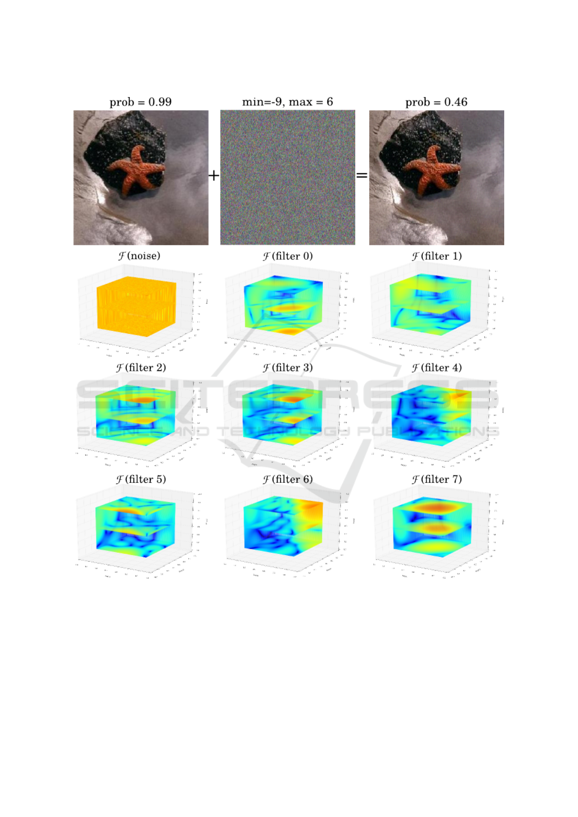
Figure 2: Analyzing the minimum noise in the frequency domain using the first 7 filters in the first layer of Googlenet obtained
from (Jia et al., 2014). The intensity of noise has been normalized so it is perceivable to human eye. The colder the color, the
smaller the spectrum (best viewed in color).
this slight change in the input can lead some of the
ConvNets to incorrectly classify the image. Also, as
the value of σ increases, the accuracy of the ConvNets
reduces. This is consistent with the explanation in
Section 2.1 in the sense that a higher value of σ in-
creases the magnitude of the all frequencies. Since
the convolution layers are not able to effectively re-
duce the noise, they are propagated through the Con-
vNet and alter the output of final convolution layer.
Second, a squashing activation function such as
tanh seems to be more tolerant against noise since
it maps the input with higher values to the outputs
with very close values. However, comparing the re-
sults obtained from IRCV and IDSIA illustrate that a
Studying Stability of Different Convolutional Neural Networks Against Additive Noise
365

Table 1: Accuracy of benchmark ConvNets on the original datasets. Trained models of AlexNet and Googlenet as well as
the architecture of Cifar10 have been obtained from (Jia et al., 2014). The architecture of gtsrb IDSIA and gstrb have been
obtained from (Ciresan et al., 2012) and our paper (will cite later), respectively.
Network accuracy (%) Network accuracy (%)
cifar10 (hing+relu) 79.8 cifar10 (soft+relu) 78.6
IRCV (GTSRB)(soft+relu) 99.01 IDSIA (GTSRB)(soft+tanh) 98.77
Alexnet (soft+relu) 87.39 Googlenet (soft+relu) 91.51
Table 2: Accuracy of the ConvNets obtained by degrading the correctly classified test images in the original datasets using
the Gaussian noise with various values for σ. For each value of σ, 100 noisy images are generated.
accuracy (%) for different values of σ
network 1 2 4 8 10 15 20 25 30 35 40
IRCV 100.0 100.0 99.8 99.3 98.8 97.4 94.3 91.2 87.8 84.5 81.4
IDSIA 99.9 99.9 99.7 99.0 98.5 97.1 94.2 91.2 88.0 84.7 81.6
CIFAR10 (hing) 99.7 99.2 98.0 94.4 91.7 84.7 71.7 59.5 47.6 37.7 30.1
CIFAR10 (soft) 99.7 99.3 98.3 95.4 93.6 88.4 77.7 67.8 58.2 49.7 42.4
alexnet 100.0 99.9 99.6 98.7 97.7 95.7 91.4 86.7 80.5 73.0 65.2
googlenet 99.8 99.7 99.5 98.5 97.8 96.0 92.7 89.2 85.1 80.3 75.2
squashing function does not necessarily make a Con-
vNet more robust.
Third, comparing the results from CIFAR10 Con-
vNet trained using softmax and hing loss functions il-
lustrate that there is not a golden rule that a specific
loss function leads to a more stable ConvNet. We ob-
serve that both ConvNets makes mistakes even when
σ = 1.
Fourth, it is observable that there is not a clear re-
lation between the size of the input and the stability of
the ConvNet. To be more specific, the size of the input
to the IDSIA and IRCV ConvNets is 48 × 48 pixels
and it is 32 × 32 pixels in the case of CIFAR10 Con-
vNets. Moreover, the size of the input of Alexnet and
Googlenet is 227 ×227 amd 224 ×224 pixels, respec-
tively. Notwithstanding, IRCV and IDSIA are more
stable than Alexnet and Googlenet. This is due to
the fact that objects in the GTSRB dataset are simpler
than the objects in the ImageNet dataset. In addition,
number of the classes in the GTSRB dataset is much
less than the number of the classes in the ImageNet
dataset. For these reasons, a 48 × 48 is enough for
IRCV and IDSIA ConvNets to accurately learn rea-
sonably stable ConvNets. In contrast, the CIFAR10
dataset contains complex objects which are presented
in small images. For this reason, some important de-
tails of the objects are missed due to down-sampling.
When the images are degraded by a strong noise, it
dramatically changes the frequency pattern which in
turn alters the classification score. In sum, stability of
a ConvNet does not solely depend on the size of the
input. Instead, choosing an appropriate input size ac-
cording to the number of the classes and complexity
of the objects in the dataset can increase the stability
of the ConvNet.
3.2 Augmenting with Noisy Images
Augmenting data by applying some transformations
on the original dataset is a common practice for in-
creasing the generalization of ConvNets. The data
augmentation procedure does not usually involve
adding noisy images to a dataset. In this experiment,
we augment the original dataset with noisy images
which are generated using the Gaussian noise. We
consider σ ∈ {1, 5, 10, 20} and 10 different noisy im-
ages are generated for each sample in the original
training set. Next, the ConvNets are fine-tuned using
the noisy datasets and they are evaluated by creating
a noisy test set as we mentioned in Section 3.1. Ta-
ble 3 and Table 4 show the accuracy of the ConvNets
obtained by applying on the original test set and the
noisy test set, respectively. As it is clear from Table
3, the ConvNets have achieved very close accuracies
compared with Table 1.
The results illustrate a considerable increase in the
accuracy of the ConvNets, especially on the images
degraded by a strong Gaussian noise. This is mainly
due to two reasons. First, the classification layer ad-
justs the decision boundary in order to correctly clas-
sify the noisy training images which increases the ac-
curacy of the ConvNets. However, it is clear that Con-
vNets also learn to reduce the effect of the noise. To
investigate this issue, we computed the frequency re-
sponse of the first layer on CIFAR10 and IRCV Con-
vNets before and after augmenting the training set
with noisy images. Then, the mean spectrum of first
layer for all the ConvNets were computed. Figure 3
illustrates the results.
The common point in both ConvNets is that the
mean spectrum of the ConvNets trained on noisy
training set is more localized than the ConvNets
trained without noisy images. In other words, a fewer
VISAPP 2017 - International Conference on Computer Vision Theory and Applications
366

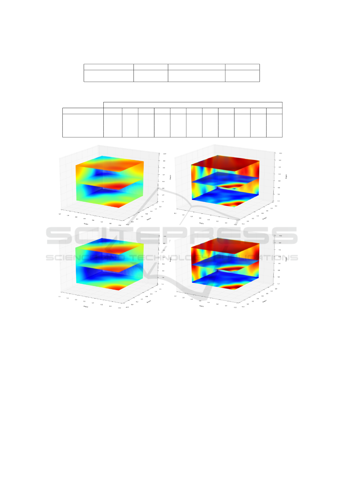
Table 3: Accuracy of ConvNets trained using the noisy datasets and tested on the original test set.
Network accuracy (%) Network accuracy (%)
IRCV (noisy) 99.29 IDSIA (noisy) 98.59
cifar10 (noisy+hing) 78.2 cifar10 (noisy+softmax) 76.6
Table 4: Accuracy of the ConvNets after augmenting the original dataset with noisy images degraded by the Gaussian noise
with σ ∈ {1, 5, 10, 20}.
accuracy (%) for different values of σ
network 1 2 4 8 10 15 20 25 30 35 40
IRCV 100.0 99.9 99.9 99.5 99.2 98.5 96.8 94.8 92.5 89.8 87.2
IDSIA 99.9 99.9 99.7 99.2 98.9 98.0 96.1 94.1 91.9 89.4 87.0
CIFAR10 (hing) 99.8 99.6 99.3 98.3 97.6 96.3 94.2 92.2 89.9 87.7 85.0
CIFAR10 (soft) 99.6 99.4 98.8 97.6 96.9 95.5 93.2 91.1 88.7 86.4 83.7
Figure 3: The mean spectrum of the first layer in the CIFAR 10 (left column) and IRCV (right column) ConvNets train using
the original (top row) and the noisy (bottom row) training datasets (Best viewed in color).
frequencies are passed through the convolution filters
trained on noisy training set. For this reason, these
ConvNets have the ability to reduce the additive noise
more effectively than the ConvNets that are trained
on the clean dataset. In sum, augmenting the dataset
using noisy images is advantageous and they help the
training algorithm to learn the convolution filters with
more concentrated spectrum.
It is worth mentioning that one can arbitrarily
change the order of the channels/filters in the first
layer and the subsequent layers accordingly without
changing the values of the output layer. This can
change the frequency response of each filter in the
third dimension. However, if we compute the fre-
quency response of the manipulated layers before and
after training by noisy samples, we still observe that
the above statement still holds true.
4 CONCLUSION
In this paper, we studied the stability of Convolutional
Neural Networks (ConvNets) against image degrada-
tion. To this end, we showed how to analyze the
convolution filters in a ConvNet by visualizing their
Fourier transform in 4-dimensions. Then, we studied
Studying Stability of Different Convolutional Neural Networks Against Additive Noise
367

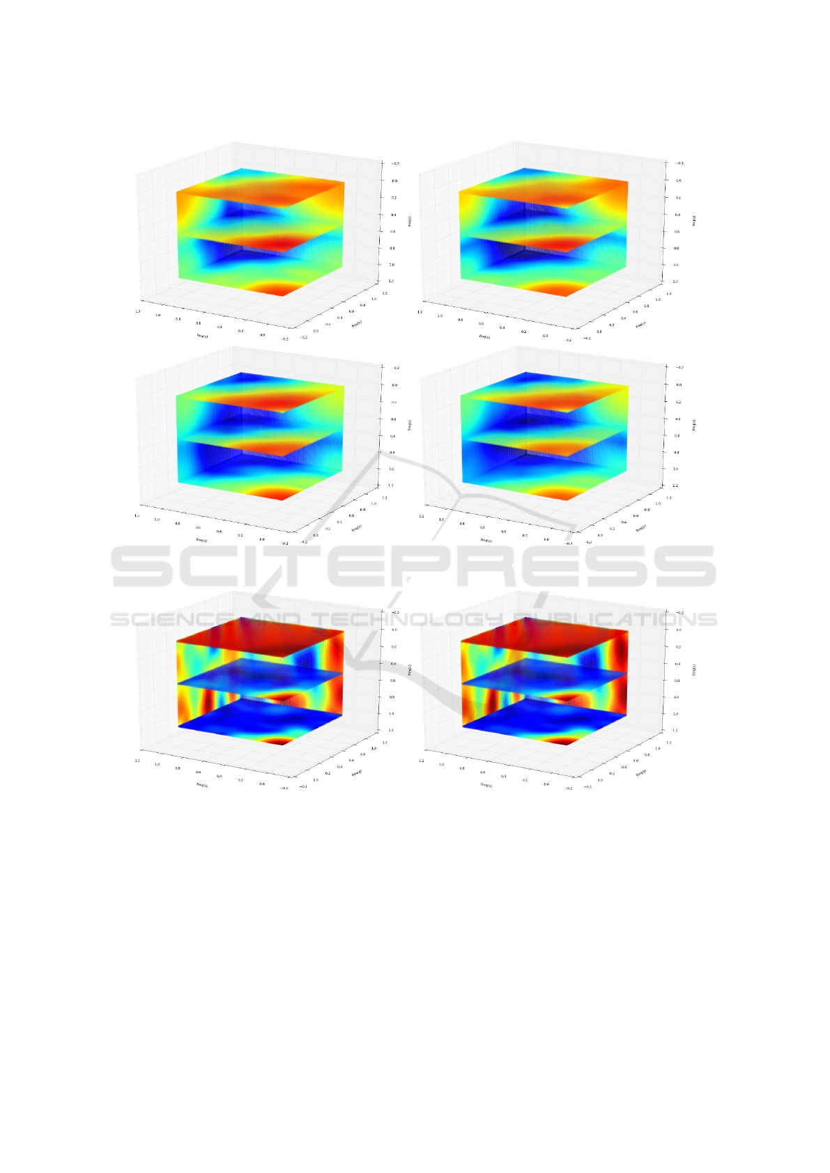
Figure 4: The mean spectrum of the first layer in the CIFAR 10 ConvNet train using the softmax (left) and the hinge (right)
loss functions. (Best viewed in color).
Figure 5: the mean spectrum of the first layer in the IDSIA ConvNet train using the original (left) and the noisy (right) training
datasets. (Best viewed in color).
why a ConvNet may make mistakes by degrading the
image using an additive noise which is barely perceiv-
able to human eye. Specifically, we illustrated that an
additive noise affects almost all the frequencies on the
image. On the other hand, analyzing the convolution
kernels in the frequency domain revealed they are not
able to effectively denoise the image and the noise is
propagated across the ConvNet that alters the classi-
fication score. Moreover, our experiments on Con-
vNets trained on different datasets showed that there
is not a golden rule to say a particular loss function or
activation function yields a more stable ConvNet. Be-
sides, the size of the input image can only affect the
performance if it is not selected based on the com-
plexity of the objects in the dataset and the number
of the classes. Next we assumed that if convolution
kernels are trained properly to have a more concen-
trated frequency response it may increase the stabil-
ity of the ConvNet. We investigated this assumption
by augmenting the training set using noisy images.
VISAPP 2017 - International Conference on Computer Vision Theory and Applications
368

Applying the ConvNets trained using noisy sets on
the noisy test sets illustrated a considerable perfor-
mance boost. We analyzed the reason by comput-
ing the mean spectrum of the convolution filters in
the first layer of the ConvNets before and after train-
ing using the noisy sets. It showed that the frequency
response of the ConvNets training on noisy sets are
more concentrated than the ConvNets trained on the
clean set.
ACKNOWLEDGMENTS
Hamed H. Aghdam and Elnaz J. Heravi are grateful
for the supports granted by Generalitat de Catalunya’s
Ag
`
ecia de Gesti
´
o d’Ajuts Universitaris i de Recerca
(AGAUR) through the FI-DGR 2015 fellowship and
University Rovira i Virgili through the Marti Franques
fellowship, respectively.
REFERENCES
Ciresan, D., Meier, U., and Schmidhuber, J. (2012). Multi-
column deep neural networks for image classifica-
tion. In IEEE Conference on Computer Vision and
Pattern Recognition, number February, pages 3642–
3649. IEEE.
Dosovitskiy, A. and Brox, T. (2015). Inverting Convolu-
tional Networks with Convolutional Networks. pages
1–15.
Fergus, R. and Perona, P. (2004). Learning Generative Vi-
sual Models from Few Training Examples :. In Com-
puter Vision and Pattern Recognition (CVPR), Work-
shop on Generative-Model Based Vision.
Girshick, R., Donahue, J., Darrell, T., Berkeley, U. C., and
Malik, J. (2014). Rich feature hierarchies for accurate
object detection and semantic segmentation. Cvpr’14,
pages 2–9.
Jia, Y., Shelhamer, E., Donahue, J., Karayev, S., Long, J.,
Girshick, R., Guadarrama, S., Darrell, T., and Eecs, U.
C. B. (2014). Caffe : Convolutional Architecture for
Fast Feature Embedding. ACM Conference on Multi-
media.
Krizhevsky, A. (2009). Learning Multiple Layers of Fea-
tures from Tiny Images. pages 1–60.
Krizhevsky, A., Sutskever, I., and Hinton, G. (2012). Im-
agenet classification with deep convolutional neural
networks. Advances in neural information processing
systems, pages 1097–1105.
Mahendran, A. and Vedaldi, A. (2014). Understanding
Deep Image Representations by Inverting Them.
Nguyen, a., Yosinski, J., and Clune, J. (2015). Deep Neural
Networks are Easily Fooled: High Confidence Predic-
tions for Unrecognizable Images. Cvpr 2015.
Simonyan, K., Vedaldi, A., and Zisserman, A. (2013).
Deep Inside Convolutional Networks: Visualising Im-
age Classification Models and Saliency Maps. arXiv
preprint arXiv:1312.6034, pages 1–8.
Stallkamp, J., Schlipsing, M., Salmen, J., and Igel, C.
(2012). Man vs. computer: Benchmarking machine
learning algorithms for traffic sign recognition. Neu-
ral Networks, 32:323–332.
Szegedy, C., Reed, S., Sermanet, P., Vanhoucke, V., and Ra-
binovich, A. (2014). Going deeper with convolutions.
pages 1–12.
Szegedy, C., Zaremba, W., and Sutskever, I. (2013). In-
triguing properties of neural networks. arXiv preprint
arXiv: . . . , pages 1–10.
Zeiler, M. D. and Fergus, R. (2013). Visualizing and Un-
derstanding Convolutional Networks. arXiv preprint
arXiv:1311.2901.
Studying Stability of Different Convolutional Neural Networks Against Additive Noise
369