Segmentation of Bone Structures by Removal of Skin and using a
Convex Relaxation Technique
José A. Pérez-Carrasco
1
, Begoña Acha
1
, C. Suárez
2
and Carmen Serrano
1
1
Signal Theory and Communications Department, University of Seville, Sevilla, Spain
2
Technological Innovation Group, Virgen del Rocío University Hospital, Sevilla, Spain
{jperez2, bacha, cserrano}@us.es, cristina.suarez.exts@juntadeandalucia.es
Keywords: CT, Bone Segmentation, Skin Extraction.
Abstract: In this paper an algorithm to extract the skin and obtain the segmentation of bones from patients in CT
volumes is described. The skin is extracted using an adaptive region growing algorithm followed by
morphological operations. The segmentation of bone structures is implemented by the minimization of an
energy function and using a convex relaxation minimization algorithm to minimize the energy term. The
cost terms in the energy function are computed using the distance between the mean and variance
parameters within bone structures in a training set and the mean and variance parameters computed locally
at each voxel position (x,y,z) in a test dataset. Several performance metrics have been computed to assess
the algorithm. Comparisons with two techniques (thresholding and level sets) have been carried out and the
results show that the algorithm proposed clearly outperform both techniques in terms of accuracy in the
delimitation results.
1 INTRODUCTION
The analysis of bone structures is interesting for
physicians, surgeons and radiologists in many
applications, such as bone fractures, cancer, analysis
of bone densities, diagnosis of some diseases
(osteoporosis, rheum, arthrosis), etc. Usually, in
these analysis, simple operations, such as
thresholding, are performed to extract bone
structures in CT 3D volumes. However, the
thresholding technique is not valid when some of
those diseases happen, as Hounsfield values within
bones may have different values as those expected.
Furthermore, Hounsfield values within bones vary
due to the different components (mainly periosteum,
compact (hard) bone, cancellous (spongy) bone and
bone marrow), making the segmentation of these
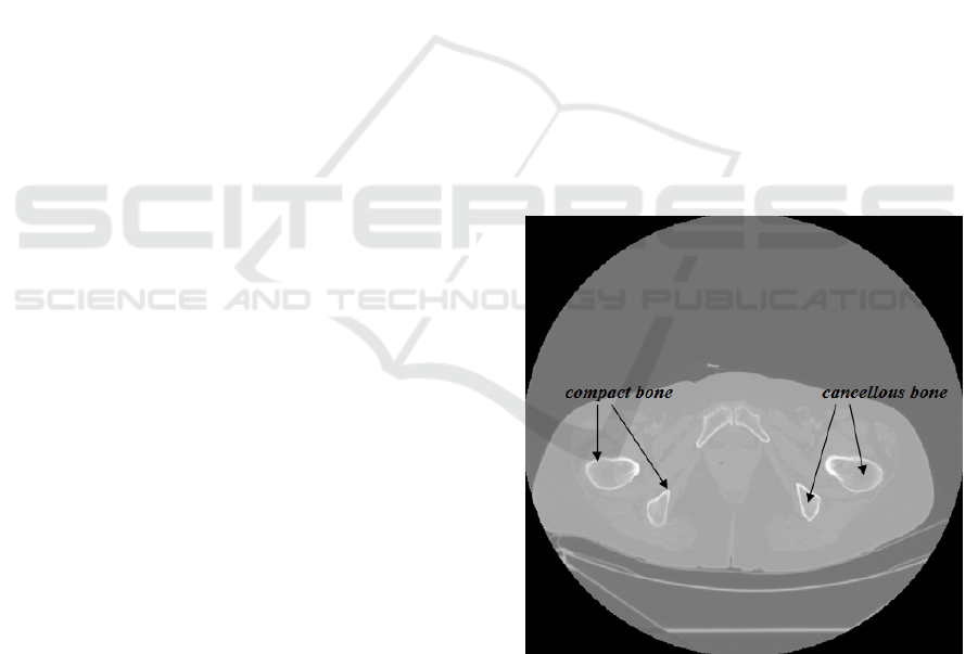
structures difficult. Fig. 1 shows a CT slice where
these Hounsfield differences can be appreciated.
Note that Hounsfield values in cancellous bone, for
instance, are quite similar to those values in
surrounding organs, making thresholding techniques
fail as they select either only the boundaries of bones
or some other soft tissues around the bone structures.
Besides, even boundaries in bone structures
(compact bone) can be difficult to be segmented due
to some of the diseases above mentioned.
Figure 1: Different parts within bones in CT volumes.
Another problem that physicians have to face is
the high computational cost when managing 3D CT
volumes. Thus, automatic algorithms able to
segment complete bone structures would be very
useful for specialists in the field, decreasing the time
in selecting them.
Many works have been presented to carry out the
Pérez-Carrasco, J., Acha, B., Suárez, C. and Serrano, C.
Segmentation of Bone Structures by Removal of Skin and using a Convex Relaxation Technique.
DOI: 10.5220/0006201105490556
In Proceedings of the 6th International Conference on Pattern Recognition Applications and Methods (ICPRAM 2017), pages 549-556
ISBN: 978-989-758-222-6
Copyright
c
2017 by SCITEPRESS – Science and Technology Publications, Lda. All rights reserved
549
segmentation of bone structures (Kang et al., 2003;
Sebastian et al., 2003; Cheng et al., 2013; Cervinka
et al., 2014; Aslan et al., 2009; Calder et al., 2011;
Kratky et al., 2008; Perez et al., 2015), being graph
cuts and level set algorithms (Kratky et al., 2008)
considered as representative of the state-of-the-art
methods. However, the main drawbacks in all these
works is that either they are focused in one or two
bone structures (hip, acetabulum, femoral head,
vertebral bodies, etc.), thus losing generality, or they
require high computational times or suffer from high
sensitivity to initialization (Kratky et al., 2008).
In this paper an algorithm to segment bone
structures is described. The procedure tries to be fast
and general to any kind of bone structures. The
paper is organized as follows: Section 2.1 describes
the extraction of the skin surface in order to facilitate
the selection of bone structures by removing
artificial structures that may have high Hounsfield
values outside the patient and reducing the areas
within each slice to be analyzed. Although there are
few works addressing the segmentation of skin in
CT volumes (Kang et al., 2014; Xiangrong et al.,
2004; Banik et al., 2010), the delimitation of the skin
can be very useful in order to facilitate the
segmentation of other organs or structures such as
liver, heart, muscle tissues, lung etc. Section 2.2
describes the algorithm developed to perform the
bone segmentation. Basically, the segmentation of
bone structures is implemented applying the
continuous max-flow algorithm by Yuan et al.,
(2010) building an energy function to be minimized.
The cost terms in the energy function are obtained
from distance images which are built by computing
the distance between the local mean and variance in
each CT voxel to the parameters mean and variance
computed from all the voxels in bone structures
within a training dataset. Section 3 shows the results
and finally, the conclusions and future work are
described.
2 METHODOLOGY
2.1 Skin Selection
In order to facilitate the segmentation of bone
structures, the first stage of the algorithm extracts
the surface skin of the patients in the CT volumes
under analysis. The common techniques to
delimitate the skin in CT volumes are based on the
use of global thresholds and edge detection
techniques (Kang et al., 2014; Zhou et al., 2004;
Banik et al., 2010). However, global thresholds are
not valid in all the cases and edge detection
techniques usually have problems with edge
delimitation and connection. As indicated in the
work by Zhou et al., (2004), skin has a depth of
about 2mms. Considering that the CT volumes
throughout this work have an xy spatial resolution of
about 0.781mm/pixel, 2mms corresponds to
approximately 3 pixels in the xy plane directions.
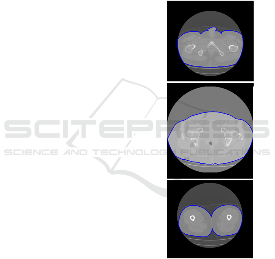
Figure 2: Skin (in blue) of three patients in different CT
slices.
The skin selection stage is performed in two
steps. In the first step, a neighbourhood-connected
region growing algorithm is applied to select inner
structures within the body. For this, some seeds
within the patient are selected. These seeds are
ICPRAM 2017 - 6th International Conference on Pattern Recognition Applications and Methods
550
selected randomly and automatically by selecting
some voxels corresponding to bone (voxels with
Hounsfield values over 1700). The inclusion
criterion only takes into account Hounsfield values
within a range specified by the user by means of two
range values. Experimentally, the best lower and
upper inclusion values were 800 and 2500,
respectively. Only voxels with values within the
range are selected if also their neighbouring voxels
have Hounsfield values within the same range. With
this algorithm, artifacts or air (like in lungs or
outside the body) are discarded. The result is a
binarized image.
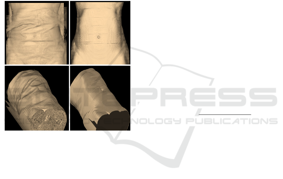
Figure 3: Examples of the 3D surface (skin) of a patient.
Left figures correspond to the surface before the skin
extraction operation. Right figures show the outer surface
of the patient.
The outer boundary of the binarized image will
correspond to the skin. Thus, in the second step, an
structure element of 3 voxels in the xy axis and 1
voxel in the z axis is employed. Using a simple
erosion morphological operation and substracting
the result to the original binarized image, the skin
can be obtained.
Fig. 2 shows the skin boundaries of three CT
slices corresponding to three different patients. Fig.
3 shows two examples of the 3D surface (skin) of a
patient. Left figures correspond to the surface before
the skin extraction operation. Right figures show the
outer surface (skin) of the patient. Note in Fig. 2 and
3 how artificial artefacts, such as sheets or bed, have
been removed.
2.2 Bone Segmentation
The algorithm for bone segmentation has three
different stages.
2.2.1 Normalization
In the first stage, a thresholding operation is
performed in order to remove soft tissue (such as fat
or some organs) with Hounsfield values below those
present in bones. To compute this threshold a set of
training CT slices were analyzed to determine the
minimum value present in all the bone structures.
More particularly, the training set was composed by
10 CT slices extracted from CTs of different patients
and different to those used in the test set.
Subsequently, a threshold was chosen under this
minimum value. The thresholding operation
guarantees that all the bone structures are maintained
in the CT slices while removing all those soft tissue
structures which could interfere in the bone structure
delimitation. The experimentally threshold obtained
had a value of 900 HU (Hounsfield Units). With this
thresholding operation all the bone structures are
still clearly visible while many of the soft tissues
have been removed.
Finally, the CT volumes are scaled with the
following scaling operation:
)_max(
Im_
Scaled_Im
settraining
Thresh
(1)
where Thresh_Im is the thresholded Image obtained
in the previous step and Scaled_im is the Image
obtained after the scaling operation. The maximum
value within the training set is used also to scale the
Dicom CT slices. Note that with this scaling
operation the Dicom slices will have values in the
range [0,1].
2.2.2 Computation of Statistical Distance
Image
In the second stage, using all the voxels within bone
structures in all the scaled CT slices belonging to the
training set, the mean and variance parameters are
extracted. This set of two parameters is denoted as
RSP (Reference Statistical Parameters). Then, for
each CT volume in the test dataset and at each voxel
position (x,y,z), the parameters mean and variance
are computed using a 5x5 local neighborhood around
the voxel position (x,y,z). Then, the Euclidean
distance from this computed set of parameters to the
reference parameter set RSP (mean and variance) is
obtained. This distance value is stored in the called
Segmentation of Bone Structures by Removal of Skin and using a Convex Relaxation Technique
551
SDI (Statistical Distance Image) image at the same
positions (x,y,z).
Fig 4 shows two slices corresponding to two
different patients (first row) and the corresponding
two SDI images obtained (second row). Note that
voxels belonging to bones have low values whereas
voxels not corresponding to bones present high
values.
2.2.3 Convex Relaxation to Implement Bone
Segmentation
In the last stage, the convex relaxation technique
proposed by Yuan et al.
(Yuan et al, 2010) is used to
perform the segmentation stage. Yuan et al.
modified the classical discrete min-cut max-flow in
graph-cut implementations by creating a continuous
domain and allowing the labeling terms to be
continuous. The fast max-flow implementation by
Yuan et al. provided a convex solution and, as
proved by Yuan et al., their implementation
outperformed the classical graph-cut techniques both
in terms of speed and accuracy. Yuan et al.
demonstrated that their fast max-flow
implementation is equivalent to the continuous s-t
min-cut problem as follows:
dxxuxCdxxCxudxxCxu
ts
xu
)()()())(1()())((min
1,0)(
(2)
where u(x) is the continuous labeling function and
s
C and
t
C
are the cost terms in the energy function.
Note that according to Eq. (1), the cost term
s
C
should take low values inside bone structures and
high outside them. On the contrary,
t
C
should take
high values inside bone structures and low values
outside them. In our experiments, Cs and Ct were
computed as follows:
Cs-1Ct
SDI))/2-(1 (Scaled_Im=Cs
(3)
The most right term in Eq. (2) is a penalty term. C(x)
is a penalty function that penalizes voxels at
boundaries with low gradients.
This C(x) function is computed as follows:
)Im(_1
)(
xScaleda
b
xC
(4)
where a and b are constants and were obtained
empirically. The parameters a and b took the values
10 and 0.2 respectively. In the third row of Fig. 4 the
cost terms Cs corresponding to two slices of two
different cases are shown.
The energy term described in Eq. (2) is
minimized using the algorithm described by Yuan et
al. in (Yuan et al., 2010).
3 RESULTS
Bone structures in 45 slices belonging to 15 different
CT volumes (and different to those in the training
set) were manually segmented by an expert and used
as groundtruth to assess the algorithm. The CT
volumes were composed on average of 250 CT
slices. The same CT slices were processed as
described in the previous section and several
evaluation metrics were computed. These metrics
have been computed in terms of TP (true positive
voxels), FP (False positive voxels), TN (true
negative voxels) and FN (False negative voxels). TP
are those voxels classified by the algorithm as bone
and also by the expert in their manual segmentation.
FP are those voxels classified as bone by the
algorithm but not by the expert. TN correspond to
voxels classified as not belonging to bones both by
the algorithm and by the groundtruth segmentation.
Finally, FN are those voxes classified as not
belonging to bones by the algorithm but they
correspond to bones according to the groundtruth.
The metrics used for the evaluation are DICE,
Jaccard, Sensitivity, Specificity, PPV and are
computed as follows:
FNFPTP
TP
2
2
Dice
(5)
FNFPTP
TP
dJaccar
(6)
FNTP
TP
ySensitivit
(7)
TNFP
TN
ySpecificit
(8)
FPTP
TP
PPV
(9)
A conventional PC (Intel ® Core ™ i7-2670QM,
CPU @ 2,20GHz, 6GB RAM) was used in all of
these evaluations.
In order to compare the results obtained by the
algorithm with other state-of-the-art methodologies,
comparisons using the same evaluation metrics with
a level set implementation and with the classical
thresholding technique have been carried out.
Particularly, the level set methodology adopted in
the experiments is the Distance Regularized Level
Set Evolution (DRLSE) implementation (Li et al,
2010). The same test dataset was used to perform the
comparisons.
In the Level-Set implementation some
configurable parameters are selected to perform the
segmentation. Particularly, the parameter values
ICPRAM 2017 - 6th International Conference on Pattern Recognition Applications and Methods
552
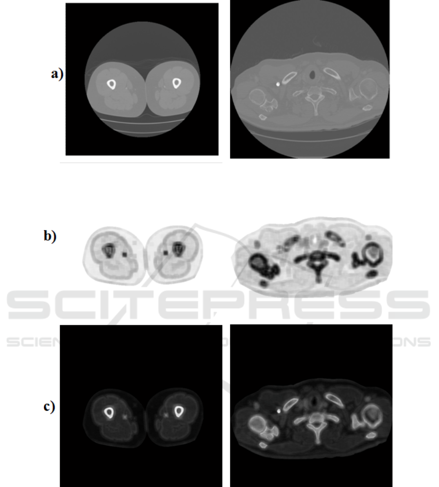
Figure 4: First row (a): Original CT slices. Second row (b): SDI images corresponding to the slices in the first row. Third
row (c): Cost Image terms used as input in the convex relaxation algorithm.
20
, timestep
5t
,
5.1
and
1
required
by the algorithm were used in our experiments. The
DRLSE algorithm was applied to the 45 scaled
dicoms (Scaled_Im) described in the previous
section.
Regarding to the thresholding implementation, a
threshold is selected and all Hounsfield values under
that threshold are set to zero. In our experiments the
threshold selected was that providing the best
results. Experimentally, using the training set, the
threshold value obtained was 1100.
Table 1 shows the evaluation metrics for the
algorithm described throughout this paper and the
two segmentation techniques above indicated. The
Segmentation of Bone Structures by Removal of Skin and using a Convex Relaxation Technique
553

average computational time required to segment one
slice for every algorithm is also indicated. Note that
the algorithm described throughout this paper was
the only providing good results, followed by the
thresholding implementation. The level set
implementation had difficulties when several bone
structures are present or when some bone structures
had diffuse boundaries or low gradient values. In
many of these cases the DRLSE algorithm required
a very high computational time (high number of
iterations) to provide acceptable results. Note,
according to Table 1, that the standard deviation
obtained in the different metrics when using the
DRLSE algorithm are high, thus showing that the
method performed very well in some slices (Dice
Coefficient of 0.94 in the best case), whereas it was
incapable of performing the segmentation in others
(Dice Coefficient of 0.04 in the worst case).
In terms of computational times, the thresholding
technique was the fastest one requiring only about
0.023 seconds to segment one slice. Considering a
CT volume composed of about 100 slices, this
would imply a processing time of only 2 seconds.
Table 1: Metrics obtained in the different experiments.
The values in the table represent the mean value of each
metric ± its standard deviation.
Thresholding DRLSE
Algorithm
proposed
Dice 0.79±0.09 0.59±0.35 0.9±0.053
Jaccard 0.66±0.13 0.49±0.34 0.83±0.087
PPV 0.80±0.13 0.52±0.37 0.86±+0.085
Sensitivity 0.80±0.16 0.94±0.21
0.97±0.049
Specificity 0.99±0.01 0.88±0.13 0.99±0.005
Computational
Time (
s
econds
per slice)
0.11±0.05 2752±657 89±6.73
In Fig. 5 the results obtained using the three
different methodologies are shown. Only some slices
are shown for visualization purposes. The red
contours correspond to the groundtruth segmentation
provided by the expert. Blue regions correspond to
the segmentation results obtained with each
algorithm. Note that the thresholding technique is
not able to select all the voxels within bones as they
present Hounsfield values under the specified
threshold. It can be also appreciated that the level set
technique had difficulties when the number of bone
structures is very high (second row, first colum) or
selected non bone tissue if it was enclosed within a
bone structure (third row, first colum).
4 CONCLUSIONS
In this paper a technique to implement the selection
of bone structures in CT volumes is described. The
first stage consists in the delimitation of the skin
(outer surface of the patient) in order to facilitate the
segmentation of the bone structures by reducing the
computational cost required. Note that the
computation of the Statistical Distance Image has a
considerable computational cost. Thus, discarding
the outer elements in the patient together with the
application of a threshold to discard soft tissues
decreases significantly the number of voxels to be
processed. Threfore, the computational time to
implement the segmentation is considerably
reduced.
A convex relaxation technique is applied using
the Histogram Distance Image as input. The convex
relaxation technique employed is the fast continuous
max-flow implementation by Yuan et al., (2010)
using the previously computed SDI image as cost
term in the energy function.
Comparison with an state-of-the-art algorithm
(DRLSE implementation) (Li et al., 2010) and the
thresholding technique, which is the preferred and
fastest technique in most of the tools used in the
clinical practice, show that the algorithm proposed
clearly outperform both techniques in terms of
accuracy in the delimitation results.
In future implementations, comparisons with
other techniques will be carried out. Note that the
performance results provided by the DRLSE
implementation were low and maybe other
techniques could be more suitable in the
segmentation of bone structures.
Besides, in future works, the two-label algorithm
described will be modified in order to identify a high
number of labels thus allowing the identification of
other kind of structures.
ACKNOWLEDGEMENTS
This research has been cofinanced by P11-TIC-7727
(Government of Andalusia, Spain) and
PT13/0006/0036RETIC (FEDER Funds and
Department of Health, Regional Government of
Andalusia).
ICPRAM 2017 - 6th International Conference on Pattern Recognition Applications and Methods
554
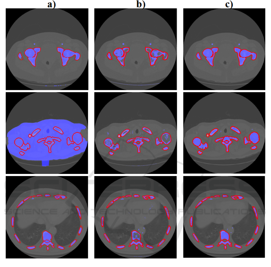
Figure 5: First Column (a) shows the results (blue regions) provided by the DRLSE algorithm. Central column (b) shows
the results (blue regions) provided by the thresholding implementation. Right column shows the results provided by the
algorithm described (blue regions). The groundtruth segmentations are contoured in red.
REFERENCES
Aslan, M.S., Ali, A., Rara, H., Arnold, B., Farag, A.A.,
Fahmi, R. and Xiang, P., 2009. 'A novel 3D
segmentation of vertebral bones from volumetric CT
images using graph cuts'. ISVC '09 Proceedings of the
5th International Symposium on Advances in Visual
Computing: Part II. Lecture Notes in Computer
Science. 5876 LNCS, pp. 519-528.
Banik, S., Rangayyan, R. M. and Boag, G. S., 2010.
'Automatic Segmentation of the Ribs, the Vertebral
Column, and the Spinal Canal in Pediatric Computed
Tomographic Images'. Journal of Digital Imaging, vol.
23, no. 3, pp. 301–322. http://doi.org/10.1007/s10278-
009-9176-x
Calder, J., Tahmasebi, A.M. and Mansouri, A.-R., 2011.
'A variational approach to bone segmentation in CT
images'. In Progress in Biomedical Optics and
Imaging Proceedings of SPIE.
Cervinka, T., Hyttinen, J. and Sievnen, H.. 2014. 'Accurate
cortical bone detection in peripheral quantitative
computed tomography images'. In IFMBE
Proceedings, pp. 289–292.
Cheng, Y., Zhou, S., Wang, Y., Guo, C., Bai, J. and
Tamura, S., 2013. 'Automatic segmentation technique
Segmentation of Bone Structures by Removal of Skin and using a Convex Relaxation Technique
555

for acetabulum and femoral head in CT images'.
Pattern Recognition, vol. 46, no. 11, pp. 2969-2984.
Kang, H.-C., Shin, Y.-G. and Lee, J., 2014. 'Automatic
segmentation of skin and bone in CT images using
iterative thresholding and morphological image
processing'. In The 18th IEEE International
Symposium on Consumer Electronics (ISCE 2014),
JeJu Island, pp. 1-2. doi: 10.1109/ISCE.2014.6884320.
Kang, Y., Engelke, K. and Kalender, W.A., 2003. 'A new
accurate and precise 3-D segmentation method for
skeletal structures in volumetric CT data'. IEEE
Transactions on Medical Imaging, vol. 22, no. 5, pp.
586–598.
Kratky, J. and Kybic, J., 2008. 'Three-dimensional
segmentation of bones from CT and MRI using fast
level sets'. In Progress in Biomedical Optics and
Imaging Proceedings of SPIE.
Li, C., Xu, C., Gui, C. and Fox, M. D., 2010. 'Distance
Regularized Level Set Evolution and its Application to
Image Segmentation'. IEEE Trans. Image Processing,
vol. 19, no. 12, pp. 3243 – 3254.
Perez, J.-A., Acha, B., and Serrano, C., 2015.
'Segmentation of Bone Structures in 3D CT Images
Based on Continuous Max-flow Optimization'. In
SPIE Proceedings Proc. SPIE 9413, Medical Imaging
2015. Image Processing, vol. 94133Y.
Sebastian, T.B., Tek, H., Crisco, J.J. and Kimia, .B., 2003.
'Segmentation of carpal bones from CT images using
skeletally coupled deformable models'. Medical Image
Analysis, vol. 7. no. 1, pp. 2-45.
Yuan, J., Bae, E. and Tai, X.-C., 2010. 'A study on
continuous max-flow and min-cut approaches'. In
Proceedings of the IEEE Computer Society
Conference on Computer Vision and Pattern
Recognition, pp. 2217–2224.
Zhou, X., Hara, T., et al., 2004. 'Automated segmentations
of skin, soft-tissue, and skeleton from torso CT
images'. Medical Imaging. Image Processing,
Proceedings of SPIE 5370 (SPIE, Bellingham, WA).
ICPRAM 2017 - 6th International Conference on Pattern Recognition Applications and Methods
556
