Malware Detection based on Graph Classiﬁcation

∗

Khanh-Huu-The Dam

and Tayssir Touili

University Paris Diderot and LIPN, Villetaneuse, France

LIPN, CNRS and University Paris 13, Villetaneuse, France

Keywords:

Machine Learning, Graph Kernel, Malware Detection, Static Analysis.

Abstract:

Malware detection is nowadays a big challenge. The existing techniques for malware detection require a huge

effort of engineering to manually extract the malicious behaviors. To avoid this tedious task of manually

discovering malicious behaviors, we propose in this paper to apply learning for malware detection. Given a

set of malwares and a set of benign programs, we show how learning techniques can be applied in order to

detect malware. For that, we use abstract API graphs to represent programs. Abstract API graphs are graphs

whose nodes are API functions and whose edges represent the order of execution of the different calls to the

API functions (i.e., functions supported by the operating system). To learn malware, we apply well-known

learning techniques based on Random Walk Graph Kernel (combined with Support Vector Machines). We can

achieve a high detection rate with only few false alarms (98.93% for detection rate with 1.24% of false alarms).

Moreover, we show that our techniques are able to detect several malwares that could not be detected by well-

known and widely used antiviruses such as Avira, Kaspersky, Avast, Qihoo-360, McAfee, AVG, BitDefender,

ESET-NOD32, F-Secure, Symantec or Panda.

1 INTRODUCTION

The number of malwares is signiﬁcantly increasing.

In 2014, there were more than 317 million new pieces

of malwares

compared to 286 millions in 2010. It is

estimated that there are nearly a million of new mal-

wares released every day. Thus, malware detection is

a big challenge.

The well-known technique to detect malware is

signature matching. It consists on searching for pat-

terns in the form of binary sequences (called signa-

tures) in the program. Signatures are manually intro-

duced in a database by experts. If a program contains

a signature in the database, it is declared as a virus. If

not, it is declared as benign. It is very easy for virus

writers to get around these signature matching tech-

niques. Indeed, obfuscation techniques can change

the structure of a malware so that it will not have a

known signature anymore while keeping its same be-

havior.

Another technique to detect malware is called dy-

namic analysis. It consists in running a malware in an

emulated environment and recording its behaviors in

real time. However, as the execution time is limited, it

∗

This work was partially funded by the FUI project AIC

2.0.

2015 Internet Security Threat Report, Volume 20,

Symantec

is hard to trigger the malicious behaviors, since these

may be hidden behind user interaction or require de-

lays.

To sidestep these limitations, static analysis tech-

niques that allow to analyse the behavior (not the syn-

tax) of the program without executing it were ap-

plied for malware detection (Bergeron et al., 1999;

Christodorescu and Jha, 2003; Kinder et al., 2010;

Song and Touili, 2013a). However, in these works,

the malicious behaviors are discovered after a man-

ual study of the assembly code of the malwares. That

task needs an enormous engineering effort and takes

an enormous amount of time. This is the reason why

only 7 malicious behaviors were considered in (Song

and Touili, 2013b), whereas there are much more ma-

licious behaviors that should be considered. Thus,

one needs techniques that prevent us from performing

this enormous amount of engineering effort of read-

ing assembly codes to discover malicious behaviors.

To solve this problem, we apply in this work

machine learning techniques for malware detection.

Given a set of malwares and a set of benign pro-

grams, we use machine learning techniques to teach

computers to automatically learn malicious behav-

iors. To do this, we need an abstract representa-

tion of programs (malicious behaviors) that we have

to learn. Following (Fredrikson et al., 2010; Babi

et al., 2011; Macedo and Touili, 2013), we use API

Dam, K-H-T. and Touili, T.

Malware Detection based on Graph Classiﬁcation.

DOI: 10.5220/0006209504550463

In Proceedings of the 3rd International Conference on Information Systems Security and Pr ivacy (ICISSP 2017), pages 455-463

ISBN: 978-989-758-209-7

455

function calls to specify malicious behaviors. Indeed,

API (which stands for Application Programming In-

terface) is a collection of functions supported by the

operating system that allow users to interact with the

system. These API functions are mediators between

programs and their running environment (user data,

network access...) that are mostly used to access or

modify the system by malware authors. According

to a statistic study

, over 5TB of different samples of

malwares, there are 527, 992 samples that did import

at least one API, compared to 21, 043 samples with

no import. Thus, API functions and their usages in

the program are crucial to specify malicious behav-

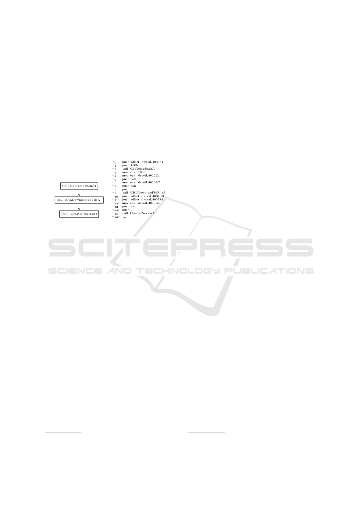
iors. Let us consider a typical malicious behavior.

(a) (b)

Figure 1: The assembly code fragment of a trojan down-

loader (b) and the API call graph (a).

Figure 1(b) is a fragment of the assembly code of a

trojan downloader. First, the function GetTempPathA

is called. This allows the program to get the loca-

tion of the temporary directory in Windows OS. Then,

the function URLDownloadToFileA is called to down-

load a ﬁle to this directory. Finally, this ﬁle is exe-

cuted by calling the function CreateProcessA. This

is a typical behavior of a trojan downloader. In order

to represent this behavior we use an API call graph,

which is a graph whose vertices are pairs (n, f ) con-

sisting of an API function f and a control point n,

and whose edges ((n, f ),(n

, f

)) express that there

is a call to the API function f at the control point

n, followed by a call to the API function f

at the

control point n

, such that between the calls f and

, there is no other call to another API function.

Figure 1(a) represents the API call graph of the be-

havior of the trojan downloader. The edge ((n

GetTempPathA),(n

, URLDownloadToFileA)) ex-

presses that at the control point n

there is a call to the

function GetTempPathA followed by the call to the

function URLDownloadToFileA at the control point

. Since the size of such graphs is huge in the case of

malwares, we apply an abstraction to reduce the size

of these graphs by merging vertices corresponding to

the same API function into one vertex associated with

http://www.bnxnet.com/

the function name. Such graphs are called abstract

API graphs.

Using this representation, we apply machine

learning techniques on graphs to learn malicious be-

haviors, and detect malwares. Support Vector Ma-

chine (SVM) is one of the most successful techniques

in machine learning. It has been applied to several

ﬁelds in pattern recognition including text analysis

and bioinformatics. In this work, we apply Sup-

port Vector Machine based learning techniques for

malware detection. The choice of Support Vector

Machine is motivated by the fact that they are very

suitable for nonvectorial data (graphs in our setting),

whereas the other well-known learning techniques

like artiﬁcial neural network, k-nearest neighbor, de-

cision trees, etc. can only be applied to vectorial data.

This SVM method is highly dependent on the choice

of kernels. A kernel is a function which returns sim-

ilarity between data. Standard kernels (including lin-

ear, polynomial, etc) handle vectorial data. However,

for nonvectorial data such as graphs, these kernels be-

come non suitable. That is the reason why we need to

use speciﬁc kernels for graphs. In this work, we use

a variant of the random walk graph kernel that mea-

sures graph similarity as the number of common paths

of increasing lengths.

The main contribution of this paper is the application

of graph kernel based learning techniques for mal-

ware detection in a completely static way (no dynamic

analysis). As far as we know, this is the ﬁrst time that

these techniques are applied for malware detection in

a static manner. We implemented our technique in a

tool and tested it on a dataset of 6291 malwares, that

are collected from Vx Heavens

, and obtained encour-

aging results. Our tool can achieve a high detection

rate with only few false alarms (98.93% for detection

rate with 1.24% of false alarms).

Moreover, we show that our techniques are able to

detect several malwares that could not be detected

by well-known and widely used antiviruses such as

Avira, Kaspersky, Avast, Qihoo-360, McAfee, AVG,

BitDefender, ESET-NOD32, F-Secure, Symantec or

Panda.

In this paper, we introduce our graph model in

Section 3. In Section 4, we discuss Support Vector

Machine techniques and the application of graph ker-

nels to our graphs in order to detect malwares. Exper-

iments are given in Section 5.

http://vxheavens.org

ICISSP 2017 - 3rd International Conference on Information Systems Security and Privacy

456

2 RELATED WORK

Machine learning techniques were applied for mal-

ware classiﬁcation in (Schultz et al., 2001; Kolter

and Maloof, 2004; Gavrilut et al., 2009; Tahan et al.,

2012; Khammas et al., 2015). However, all these

works use either a vector of bits (Schultz et al., 2001;

Gavrilut et al., 2009) or n-grams (Kolter and Maloof,

2004; Tahan et al., 2012; Khammas et al., 2015) to

represent a program. Such vector models allow to

record some chosen information from the program,

they do not represent the program’s behaviors. Thus

they can easily be fooled by standard obfuscation

techniques, whereas our API graph representation is

more precise and represents the API call behavior of

programs and can thus resist to several obfuscation

techniques.

(Ravi and Manoharan, 2012) use sequences of API

function calls to represent programs and learn mali-

cious behaviors. Each program is represented by a

sequence of API functions which are captured while

executing the program. (Rieck et al., 2008) uses as

model a string that records the number of occurences

of every function in the program’s runs. Our model

is more precise and more robust than these two rep-

resentations as it allows to take into account several

API function sequences in the program while keep-

ing the order of their execution. Moreover, (Ravi and

Manoharan, 2012) and (Rieck et al., 2008) use dy-

namic analysis to extract a program’s representation.

As said above, our API graph extraction is done in a

static way.

(Christodorescu et al., 2007; Kinable and

Kostakis, 2011; Fredrikson et al., 2010; Macedo

and Touili, 2013; Elhadi et al., 2015) represent pro-

grams using graphs similar to our API call graphs.

(Christodorescu et al., 2007; Fredrikson et al., 2010;

Macedo and Touili, 2013) use graph mining algo-

rithms to compute the subgraphs that belong to mal-

wares and not to benign programs and they assume

that these correspond to malicious behaviors. We do

not make such assumption as two malwares may not

have any common subgraphs. Moreover, (Christodor-

escu et al., 2007; Fredrikson et al., 2010) use dynamic

analysis to compute the graphs, whereas our graph

extraction is made statically. (Kinable and Kostakis,

2011) uses clustering techniques. This approach de-

pends highly on the number of clusters that has to be

provided. The performance degrades if the number

of clusters is not optimal. (Elhadi et al., 2015) uses

graph similarity based on comparison of the longest

common subsequences. Our graph kernels are more

robust since, to compare graphs, we take into account

all paths existing in the graph.

(Nikolopoulos and Polenakis, 2016) use graphs sim-

ilar to our API graphs where each node corresponds

to a group of API function calls. Our graphs are more

precise since we do not group API functions together.

Moreover, (Nikolopoulos and Polenakis, 2016) uses

dynamic analysis to extract graphs, whereas our tech-

niques are static. Furthermore, they deﬁne their own

similarity metric to classify malwares whereas we use

the well-known SVM method for malware classiﬁca-

tion.

(Kong and Yan, 2013; Xu et al., 2013) use graphs

where nodes are functions of the program (either API

functions or any other function of the program). Such

representations can easily be fooled by obfuscation

techniques such as function renaming. Moreover,

these works do not use graph kernel based SVM to

classify graphs.

Graph kernel based SVM for malware detection is

used in (Anderson et al., 2011; Wagner et al., 2009).

(Wagner et al., 2009) uses graphs to represent the sys-

tem’s behaviors (system commands, process IDs...)

not the program’s behaviors as we do. This approach

can only be done by dynamic analysis. Moreover,

(Wagner et al., 2009) uses a kind of random walk

graph kernel based SVM to learn malicious behav-

iors. Our random walk graph kernel is more precise

for graph comparison since our kernel takes into ac-

count path lengths in graphs in a more precise way.

As for (Anderson et al., 2011), they use graphs to rep-

resent the order of execution of the different instruc-

tions of the programs (not only API function calls).

Our API graph representation is more robust. Indeed,

considering all the instructions in the program makes

the representation very sensitive to basic obfuscation

techniques. Moreover, (Anderson et al., 2011) uses

graph kernel based SVM to learn malicious behaviors.

They use the Gaussian and spectral kernels which al-

low them to compare the structure of graphs. Our

random walk graph kernel compares the paths of the

graph instead. This allows us to compare the behav-

iors of the programs where a behavior is a sequence

of API functions.

3 BINARY CODE MODELING

Malwares are usually executables, i.e., binary codes.

Thus, we show in this section how to extract an

API call graph from a binary code. Given a binary

code, we apply the disassembly tools IDA Pro (Ea-

gle, 2011), Jakstab (Kinder and Veith, 2008) and

BePum (Nguyen et al., 2013) to extract a control ﬂow

graph (CFG) (a standard representation of programs

in the program analysis community). Then, we use

this CFG to construct an API call graph. Since mal-

Malware Detection based on Graph Classiﬁcation

457

wares contain a huge number of instructions in their

codes, the obtained API call graphs are huge (more

than 854 vertices in our dataset). Thus, the learn-

ing technique we applied took a lot of time. To be

more efﬁcient, we introduce an abstraction of the API

call graph, called abstract API graph, that consists in

merging the vertices of the API call graph that corre-

spond to the same API function. In this section, we

ﬁrst recall the deﬁnition of a control ﬂow graph, then

we deﬁne API call graphs and abstract API graphs,

and show how to compute them from the CFG of the

program.

3.1 Control Flow Graph

A Control Flow Graph (CFG) is a tuple G = (N, I,E),

where N is a ﬁnite set of vertices, I is a ﬁnite set of

assembly instructions in a program, and E : N × I ×N

is a ﬁnite set of edges. Each vertex corresponds to

a control point of the program. Each edge connects

two control points in the program and is associated

with an assembly instruction. An edge (n

,i,n

) in

E expresses that in the program, the control point n

is followed by the control point n

and is associated

with the instruction i.

3.2 API Call Graph

Let A be the set of all API functions that are called

in the program. An API call graph is a directed graph

api

= (V

api

), where V

api

: N × A is a ﬁnite set

of vertices and E

api

: (N × A)×(N × A ) is a ﬁnite set

of edges. We deﬁne the labeling function ` : V

api

→

A such that `((n, f )) = f (the label of a vertex is its

corresponding API function). A vertex (n, f ) means

that at a control point n, a call to the API function f

is made. An edge ((n

, f

),(n

, f

)) in E means that

the API function f

called at the control point n

executed after the API function f

called at the control

point n

. Moreover, between the control points n

and

, there is no call to another API function.

3.3 Abstract API Graph

As the size of the previous graph is quite huge in the

case of malwares, we apply an abstraction to reduce

the size of the API call graphs by merging vertices

corresponding to the same API function in one vertex

associated with the function name, i.e., the vertices

, f ), (n

, f ), ..., (n

, f ) are merged in a single vertex

labeled by the API function f . By doing that, the size

of graphs in our dataset is reduced by about a quarter

while the accuracy is not changed so much. Thus, all

our experiments are made on abstract API graphs (not

on API call graphs).

Given an API call graph G

api

= (V

api

), an

abstract API graph is a directed graph G

aapi

), where V

aapi

⊆ A is a set of vertices,

and E

aapi

is a set of edges. Each vertex is labeled

by an API function. There is an edge ( f

, f

) ∈ E

aapi

if there exist control points n

and n

, such that

((n

, f

),(n

, f

)) is in G

api

. We deﬁne the labeling

function ` : V

aapi

→ A such that `(v) = v for every

v ∈ V

aapi

(the label of a vertex is its corresponding

API function).

4 LEARNING MALICIOUS

BEHAVIORS

In order to detect malicious behaviors, we cast the

problem of malware detection as graph classiﬁcation.

The goal is to check whether a given unseen data

belongs to the positive (malign) or the negative (be-

nign) class. For that purpose, we build a classiﬁer,

that decides about this class membership using a la-

beled training set. The latter includes positive as well

as negative examples.

In what follows, we discuss the application of

kernel-based support vector machines (SVMs) in mal-

ware detection. The choice of SVMs is motivated by

their well established generalization ability in many

pattern classiﬁcation problems, especially those in-

volving small or mid size training databases. More

importantly, and in contrast to other well known train-

ing algorithms, SVMs are very suitable when han-

dling semi-structured and non-vectorial data (such

as graphs), through the use of well dedicated kernel

functions as shown subsequently.

4.1 Kernel-based Support Vector

Machines

In this section, we recall the basic deﬁnitions used

in kernel-based support vector machine training and

show how we apply it for learning malicious behav-

iors. We refer the reader to (Burges, 1998) for a tuto-

rial on this technique.

Let’s consider a collection of training data

{(x

)}

i=1

; with x

being a feature in a vector

space and y

its class label in {−1,+1}. Support

Vector Machine (SVM) training consists in ﬁnding

an optimal classiﬁer (hyperplane), denoted h, that

separates labeled data in {(x

)}

while maximizing

their margin. Considering w as the normal of that

Abstract API graph associated to a new program

ICISSP 2017 - 3rd International Conference on Information Systems Security and Privacy

458

hyperplane h, the SVM decision function of h can be

written as

h(x) = w

x + b, (1)

here x

stands for the transpose of x, w =

∑

i=1

(with {α

}

being the SVM training parameters) and

b is a shift. When training data are linearly separable,

the hyperplane h guarantees that y

+ b) ≥ 1,

∀i ∈ {1, .. ., n}.

In the context of graph classiﬁcation, the train-

ing set corresponds to {(G

)}

with G

being an

abstract API graph and y

= +1 if G

is malign and

= −1 otherwise. As graphs are non-vectorial data,

we consider a function φ(.) which maps graphs into a

high dimensional vector space (denoted H ) that also

guarantees the linear separability of training data. Us-

ing φ, the decision function h, associated to graphs,

can be written as

h(G) = w

φ(G)+ b =

∑

i=1

hφ(G

),φ(G)i +b, (2)

where w =

∑

i=1

φ(G

) and hφ(G

),φ(G)i deﬁnes

an inner product. Instead of φ, one may use the in-

ner product hφ(G

),φ(G)i and this deﬁnes a kernel

function (denoted κ(G

,G)). Conversely, a symmet-

ric function κ deﬁnes an inner product, in some H , iff

κ is positive semi-deﬁnite(Vishwanathan et al., 2010).

With this kernel deﬁnition, Equation 2 can be rewrit-

ten as

h(G) =

∑

i=1

κ(G

,G) + b. (3)

Using (3) and a threshold τ, a given graph G is as-

signed to the malicious (resp. benign) class iff h(G) ≥

τ (resp. h(G) < τ) for τ ∈ R (see Figure 4 for results

w.r.t. different values of τ). The value of h(G) is also

seen as a conﬁdence score of a given sample G w.r.t

the positive class.

In the remainder of this section, we deﬁne the ker-

nel function κ (used in SVMs) that implicitly maps

non-vectorial data (particularly graphs) into a high

dimensional vector space H ; this guarantees the lin-

ear separability of data in the mapping space H and

also provides a relevant similarity measure between

graphs in order to achieve malicious behavior detec-

tion and recognition effectively.

4.2 Random Walk Graph Kernel

Given two graphs G = (V, E) and G

= (V

), the

random walk graph kernel (RDW) – introduced in

artner et al., 2003) – deﬁnes a similarity κ(G, G

as the number of common walks in their product

graph G

. The latter is a graph over pairs of

vertices from G and G

; two vertices in G

are

connected by an edge iff the corresponding ver-

tices in G and G

are both connected. More for-

mally, the product graph G

= (V

) is deﬁned

as V

= {(v, v

)|v ∈ V and v

∈ V

: `(v) = `(v

)}

and E

= {((v, v

),(w,w

))|(v,w) ∈ E,(v

) ∈ E

`(v) = `(v

) and `(w) = `(w

)}, here ` is a label-

ing function

With this product graph, RDW is deﬁned as

κ(G,G

) :=

∑

k=0

µ(k)q

, (4)

here

is the adjacency matrix of the product graph G

and A

is recursively deﬁned as A

= A

k−1

(resp. q

) is a vector with as many entries as ver-

tices in G

(resp. G

). which characterizes the acces-

sibility of vertices in G

(resp. G

). In practice, p

and q

are set to uniform distributions, T is the max-

imum length of a random walk,

µ(k) = λ

∈ [0, 1] is a coefﬁcient that controls the im-

portance of the length in random walks.

As a vertex in the product graph G

corresponds to

a pair of vertices (with the same API function) in the

call graphs G

, G

, a path (with any length k ≥ 0) in

represents a sequence of common API calls that

appears in both graphs G

and G

; this characterizes

a common behavior occurring in the two underlying

programs. With this RDW kernel, the similarity be-

tween training and test data is well captured as shown

through SVM classiﬁcation experiments in the fol-

lowing section.

5 EXPERIMENTS

5.1 Dataset and Evaluation Measures

In order to evaluate the performance of our kernel-

based SVMs, we collect a dataset of 6291 malware

samples from Vx Heavens and 2323 benign programs

from system ﬁles and applications in Windows OS

and Cygwin. The proportion of malware categories

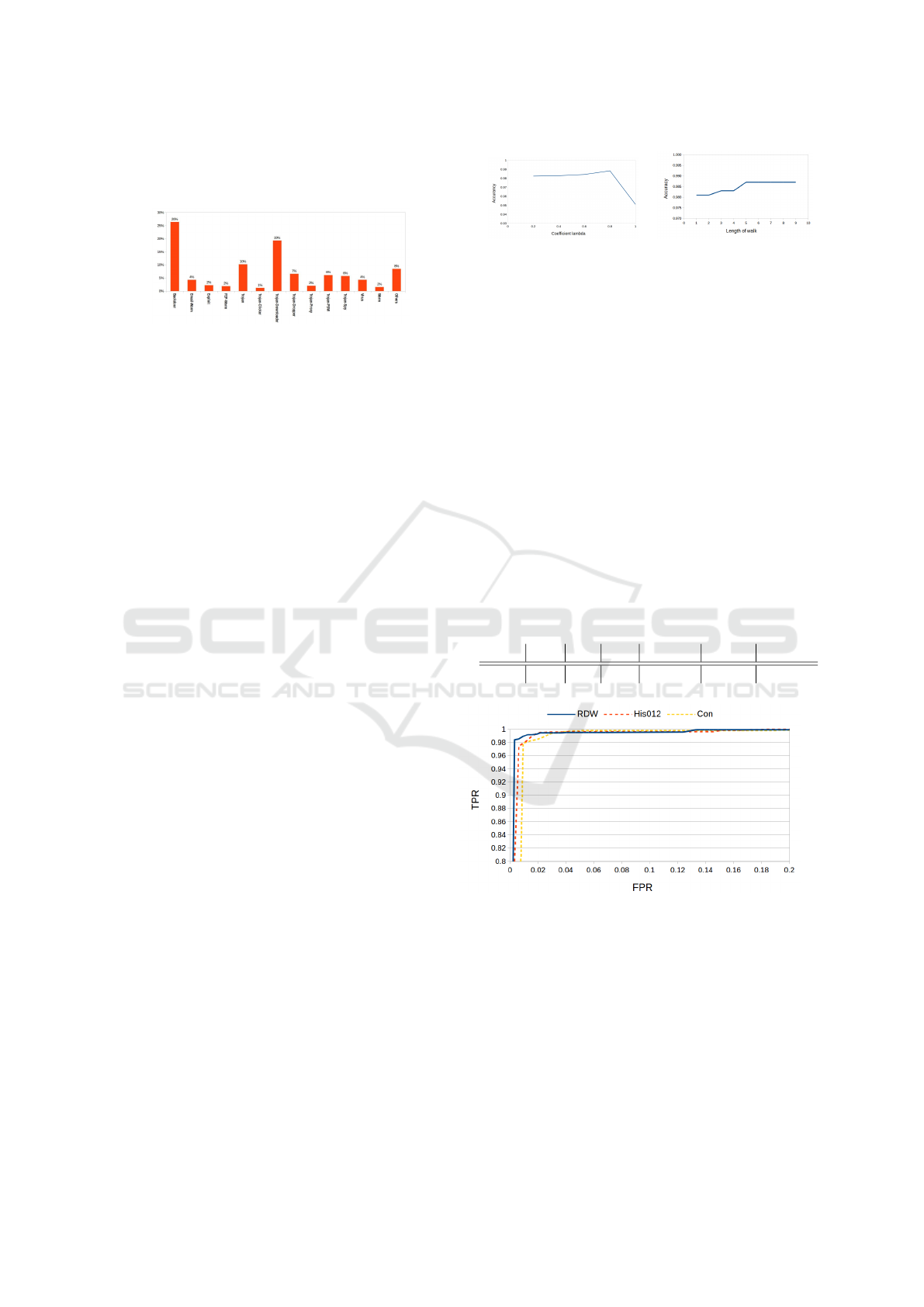
is shown in Figure 2. The dataset randomly split

into two partitions, a training and a testing partition.

For training partition, the quantity of malwares and

benign programs is balanced with 2000 samples for

each. The testing set consists of 4291 malwares and

323 benign programs. In order to capture the variabil-

ity of the dataset, we use 5 random splits of training

and test data, then we take the average of the perfor-

mances. Computing the kernel matrix for the whole

In the context of the abstract API graph, the label of a

vertex is an API function.

Malware Detection based on Graph Classiﬁcation

459

dataset of 8614 graphs takes 3 days, but this is an of-

ﬂine computation. Online computation to classify a

new program with size 15 KB takes 15 seconds.

Figure 2: The malware distribution in the dataset, showing

the percentage of different categories with respect to the to-

tal number of malware ﬁles.

Using this dataset, we consider two subtasks for eval-

uation.

• Malware detection. This is the principal task of

our contribution. We train a single monolithic

SVM classiﬁer (h) using positive and negative

data in the training set. This classiﬁer h is used

in order to check whether a given test graph G be-

longs to the malign (positive) or benign (negative)

class depending on the sign of h(G), i.e., τ = 0.

• Malware category recognition. As a secondary

task, the goal is to recognize the category of a

given malign graph G. For that purpose, we train

for each category (denoted c), a “one-versus-all”

SVM classiﬁer h

that separates graphs belonging

to the c

category from all others. Given a test

graph G with h(G) ≥ 0, the category of G corre-

sponds to argmax

(G).

In both tasks, we plug the RDW kernel in SVMs and

we use the widely known library (LIBSVM)(Chang

and Lin, 2011) for SVM training.

We evaluate the performance of our SVM classi-

ﬁers (h and {h

}

) using well known measures: true

positive and false positive rates respectively deﬁned

as TPR = TP/(TP + FN) and FPR = FP/(TN + FP);

here TP, TN, FP, FN respectively denote true pos-

itives, true negatives, false positives and false nega-

tives obtained after SVM classiﬁcation. We also re-

port BCR (balanced correctness rate) as one minus

the average between false positive and false negative

rates (BCR = 1 − (FPR + FNR)/2) where the false

negative rate FNR = FN/(FN + TN). Finally, we re-

port the overall accuracy ACC = (TP + TN)/(TP +

TN +FP + FN). For all these measures, higher values

of TPR, BCR, ACC (with small values of FPR) imply

better performances.

5.2 Performances and Comparison

Performances of Malware Detection. Firstly, we

measure the performance of the RDW kernel (com-

(a) (b)

Figure 3: This diagram shows the evolution of the Accuracy

w.r.t λ (a) and T (b) in the RDW kernel.

bined with SVM) w.r.t different walk lengths (i.e.,

w.r.t parameter T in Eq. 4) and different values of

coefﬁcient λ to control the importance of the length

in random walks in µ(k) = λ

of Eq. 4. Figure 3(a)

shows that the classiﬁcation accuracy ACC increases

as λ increases from 0.2 to 0.8, then it decreases af-

ter reaching the max value at λ = 0.8. Figure 3(b)

shows that as T increases, the classiﬁcation accuracy

ACC increases and stabilizes when T reaches 5 ran-

dom walks. Following these results, T is ﬁxed to 5

and λ is ﬁxed to 0.8 in all the remaining experiments;

with this setting, detection rates (TPR), reported in

Table 1 reach 98.93%, with a false positive rate FPR

of 1.24%.

Table 1: This table shows the performances of RDW kernel.

We obtain these results by averaging the results of 5 runs,

each run corresponds to a random split of the dataset into

training and test data.

TP TN FP FN TPR FPR ACC

4245 319 4 46 98.93% 1.24% 98.91%

Figure 4: This ﬁgure shows true positive rates vs. false

positive rates of our method and its comparison against

the two baseline kernels: structured histogram intersection

and convolution kernels (referred to as His012 and Con).

These results show that RDW achieves the best true positive

rate (around 99% with a small FPR; around 1%) compared

to histogram intersection and convolution kernels (which

achieve a TPR of 98%).

Secondly, we compare the performance of the RDW

kernel against two widely used baseline kernels for

graph comparison: (i) convolution kernel and (ii)

structured histogram intersection kernel. Given two

graphs G = (V,E) and G

= (V

), the convolu-

ICISSP 2017 - 3rd International Conference on Information Systems Security and Privacy

460

tion kernel introduced in (Haussler, 1999) for semi-

structured data (including graphs), is deﬁned as

κ(G,G

) =

|V |×|V

∑

v∈V

∑

∈V

{`(v)=`(v

)}

, here 1

{}

corresponds to the indicator function.

The second baseline kernel – structured histogram in-

tersection – is deﬁned as

κ(G,G

) = κ

(G,G

) + κ

(G,G

) + κ

(G,G

), (5)

here κ

(G,G

), κ

(G,G

) and κ

(G,G

) correspond to

standard histogram intersection kernels associated to

cliques of order 0, 1 and 2 respectively (i.e., vertices,

edges and connected subgraphs with 3 vertices). Fol-

lowing (Barla et al., 2003; Maji et al., 2008), these

three kernels are deﬁned as

(G,G

) =

∑

i=1

min(g

(G,`

),g

))

(G,G

) =

∑

i, j=1

min(g

(G,`

),g

))

(G,G

) =

∑

i, j,k=1

min(g

(G,`

),g

)),

(6)

here L is |A|, i.e., is the number of API functions in

the program. g

(G,`

) is the probability of occurrence

of label `

in G, i.e., g

(G,`

) =

|V |

∑

v∈V

{`(v)=`

}

Similarly, g

(G,`

) (resp. g

(G,`

)) corre-

sponds to the probability of occurrence of edges with

labels (`

) (resp. connected triplet of vertices with

labels (`

)).

Figure 4 shows the evolution of the true positive rate

(TPR) and the false positive rate (FPR) w.r.t. different

and increasing values of τ, taken from min to max

value of h(G), i.e., τ ∈ [−4,6]. The interesting part of

these diagrams corresponds to small values of FPR;

indeed, for reasonably small and comparable FPRs,

our method based on the RDW kernel has high TPRs

and it clearly overtakes the convolution kernel as well

as structured histogram intersection kernel.

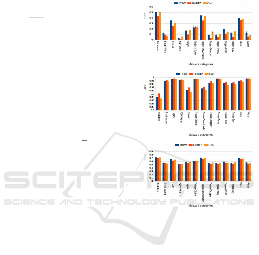
Performances of Malware Category Recognition.

Again, given a graph G (with h(G) ≥ 0), the goal is to

assign it to one of 13 malware categories (Backdoor,

Email-Worm, Exploit, P2P-Worm, Trojan, Trojan-

Clicker, Trojan-Downloader, Trojan-Dropper, Trojan-

Proxy, Trojan-PSW, Trojan-Spy, Virus and Worm)

based on argmax

(G) (thanks to Equation 3). Fig-

ure 5 shows the classwise TPR, Accuracy and BCR

rates of our RDW kernel and its comparison against

the two other baseline kernels.

Comparison with Well-known Antiviruses. We

compare the performance of our method with dif-

ferent existing antiviruses including Avira, Kasper-

sky, Avast, Qihoo-360, McAfee, AVG, BitDefender,

ESET-NOD32, F-Secure, Symantec and Panda. Since

known antiviruses update their signature database as

soon as a new malware is known, in order to have

a fair comparision with these antiviruses, we need to

consider new malwares. For this, we use three gener-

ators to create new malwares: NGVCK, RCWG and

(a)

(b)

(c)

Figure 5: This ﬁgure shows class-by-class malware cate-

gory recognition performances of our RDW-based method

and the two other baselines kernels on 13 malware cate-

gories. Fig. (a), (b) and (c) show detection rate (TPR), ac-

curacy and balanced correctness rate (BCR) for each mal-

ware category and their variances. Our method reaches a

BCR of 60% while histogram intersection and convolution

kernels obtain 58% and 59% respectively. Results are aver-

aged over ﬁve experimental runs.

VCL32. The latter are able to create sophisticated

malwares with morphing code and other features to

avoid being detected by antiviruses. In total, we

generate 180 new malwares by RCWG, VCL32 and

NGVCK generators. After training our SVM classi-

ﬁer on the training set, we are able to detect 100%

of new malwares while none of the well known an-

tiviruses can detect all of them. The results are shown

in Table ??.

Malware Detection based on Graph Classiﬁcation

461

Table 2: This table shows a comparison of our method

against well-known antiviruses. Our tool achieves a detec-

tion rate of 100%.

Antivirus Detection Rates Antivirus Detection Rates

Our tool 100% Panda 19%

Avira 16% Kaspersky 81%

Avast 87% Qihoo-360 96%

McAfee 96% AVG 82%

BitDefender 87% ESET-NOD32 87%

F-Secure 87% Symantec 14%

6 CONCLUSION

The main contribution of this paper is the applica-

tion of graph kernel based learning techniques for

malware detection in a completely static way (no dy-

namic analysis). As far as we know, this is the ﬁrst

time that these techniques are applied for malware

detection in a static manner. We introduced an auto-

matic malware detection algorithm based on SVMs.

First, we use static analysis in order to create ab-

stract API graphs from control ﬂow graphs. Then, we

build SVMs that learn the malicious behaviors from

these API graphs and achieve malware detection and

recognition. These SVMs are built upon a well ded-

icated random walk graph kernel (RDW) that mea-

sures graph similarity as the number of common paths

of increasing lengths and characterizes common ma-

licious behaviors through training and test data. The

use of this kernel is clearly appropriate as it allows us

to handle non-vectorial data (i.e., graphs) without any

explicit generation of features on these graphs. Exper-

iments show that our RDW-based classiﬁer achieves

a TPR of almost 99% with only 1.24% FPR for mal-

ware detection and an accuracy of 96.55% for mal-

ware category recognition. Compared to other ker-

nels (such as histogram intersection and convolution),

our RDW based method obtains the best classiﬁcation

performances.

Note that we could have extracted vectorial features

from graphs and then applied other learning tech-

niques such as ANNs, but this would have led to loss

of information. Thus, we believe that applying graph

kernel based SVMs is the best choice to learn our ma-

licious behavior graphs.

REFERENCES

Anderson, B., Quist, D., Neil, J., Storlie, C., and Lane,

T. (2011). Graph-based malware detection using

dynamic analysis. Journal in Computer Virology,

7(4):247–258.

Babi

c, D., Reynaud, D., and Song, D. (2011). Malware

analysis with tree automata inference. CAV’11.

Barla, A., Odone, F., and Verri, A. (2003). Histogram inter-

section kernel for image classiﬁcation. In ICIP 2003.

Bergeron, J., Debbabi, M., Erhioui, M., and Ktari, B.

(1999). Static analysis of binary code to isolate mali-

cious behaviors. In WET ICE ’99.

Burges, C. J. C. (1998). A tutorial on support vector ma-

chines for pattern recognition. Data Min. Knowl. Dis-

cov., 2(2).

Chang, C.-C. and Lin, C.-J. (2011). Libsvm: A library for

support vector machines. ACM Transactions on Intel-

ligent Systems and Technology, 2. Software available

at http://www.csie.ntu.edu.tw/ cjlin/libsvm.

Christodorescu, M. and Jha, S. (2003). Static analysis of

executables to detect malicious patterns. SSYM’03.

Christodorescu, M., Jha, S., and Kruegel, C. (2007). Mining

speciﬁcations of malicious behavior. ESEC-FSE ’07.

ACM.

Eagle, C. (2011). The IDA Pro Book. No Starch Press, 2nd

edition.

Elhadi, E., Maarof, M. A., and Barry, B. (2015). Improving

the detection of malware behaviour using simpliﬁed

data dependent api call graph.

Fredrikson, M., Jha, S., Christodorescu, M., Sailer, R., and

Yan, X. (2010). Synthesizing near-optimal malware

speciﬁcations from suspicious behaviors. SP ’10.

artner, T., Flach, P., and Wrobel, S. (2003). On graph

kernels: Hardness results and efﬁcient alternatives. In

Learning Theory and Kernel Machines.

Gavrilut, D., Cimpoesu, M., Anton, D., and Ciortuz, L.

(2009). Malware detection using perceptrons and sup-

port vector machines. In 2009 Computation World:

Future Computing, Service Computation, Cognitive,

Adaptive, Content, Patterns. IEEE.

Haussler, D. (1999). Convolution kernels on discrete struc-

tures.

Khammas, B. M., Monemi, A., Bassi, J. S., Ismail, I., Nor,

S. M., and Marsono, M. N. (2015). Feature selection

and machine learning classiﬁcation for malware de-

tection. Jurnal Teknologi, 77.

Kinable, J. and Kostakis, O. (2011). Malware classiﬁcation

based on call graph clustering. J. Comput. Virol., 7(4).

Kinder, J., Katzenbeisser, S., Schallhart, C., and Veith, H.

(2010). Proactive detection of computer worms using

model checking. Dependable and Secure Computing,

IEEE Transactions on, 7(4).

Kinder, J. and Veith, H. (2008). Jakstab: A static analy-

sis platform for binaries. In Gupta, A. and Malik, S.,

editors, Computer Aided Veriﬁcation, volume 5123.

Kolter, J. Z. and Maloof, M. A. (2004). Learning to detect

malicious executables in the wild. KDD ’04.

Kong, D. and Yan, G. (2013). Discriminant malware dis-

tance learning on structural information for automated

malware classiﬁcation. In Proceedings of the 19th

ACM SIGKDD international conference on Knowl-

edge discovery and data mining.

Macedo, H. and Touili, T. (2013). Mining malware spec-

iﬁcations through static reachability analysis. In ES-

ORICS 2013.

ICISSP 2017 - 3rd International Conference on Information Systems Security and Privacy

462

Maji, S., Berg, A., and Malik, J. (2008). Classiﬁcation us-

ing intersection kernel support vector machines is ef-

ﬁcient. In CVPR 2008.

Nguyen, M. H., Nguyen, T. B., Quan, T. T., and Ogawa,

M. (2013). A hybrid approach for control ﬂow graph

construction from binary code. In APSEC 2013, vol-

ume 2.

Nikolopoulos, S. D. and Polenakis, I. (2016). A graph-

based model for malware detection and classiﬁcation

using system-call groups. Journal of Computer Virol-

ogy and Hacking Techniques, pages 1–18.

Ravi, C. and Manoharan, R. (2012). Malware detection us-

ing windows api sequence and machine learning. In-

ternational Journal of Computer Applications, 43.

Rieck, K., Holz, T., Willems, C., Dussel, P., and Laskov, P.

(2008). Learning and classiﬁcation of malware behav-

ior. DIMVA ’08.

Schultz, M., Eskin, E., Zadok, E., and Stolfo, S. (2001).

Data mining methods for detection of new malicious

executables. In S P 2001.

Song, F. and Touili, T. (2013a). Ltl model-checking for mal-

ware detection. In Piterman, N. and Smolka, S., ed-

itors, Tools and Algorithms for the Construction and

Analysis of Systems, volume 7795.

Song, F. and Touili, T. (2013b). Pommade: Pushdown

model-checking for malware detection. ESEC/FSE

2013.

Tahan, G., Rokach, L., and Shahar, Y. (2012). Mal-id:

Automatic malware detection using common segment

analysis and meta-features. J. Mach. Learn. Res.,

13(1).

Vishwanathan, S. V. N., Schraudolph, N. N., Kondor, R.,

and Borgwardt, K. M. (2010). Graph kernels. J. Mach.

Learn. Res., 11.

Wagner, C., Wagener, G., State, R., and Engel, T. (2009).

Malware analysis with graph kernels and support vec-

tor machines. In MALWARE 2009. IEEE.

Xu, M., Wu, L., Qi, S., Xu, J., Zhang, H., Ren, Y., and

Zheng, N. (2013). A similarity metric method of ob-

fuscated malware using function-call graph. Jour-

nal of Computer Virology and Hacking Techniques,

9(1):35–47.

Malware Detection based on Graph Classiﬁcation

463