WAVE: A 3D Online Previewing Framework for Big Data Archives

Nicholas Tan Jerome, Suren Chilingaryan, Andrei Shkarin, Andreas Kopmann,

Michael Zapf, Alexander Lizin and Till Bergmann

Institute for Data Processing and Electronics (IPE), Karlsruhe Institute of Technology (KIT),

Eggenstein-Leopoldshafen, Germany

Keywords:

Web-based Visualization, Scientiﬁc Visualization, Multi-resolution Slicemap, Visual Data Browsing.

Abstract:

With data sets growing beyond terabytes or even petabytes in scientiﬁc experiments, there is a trend of keeping

data at storage facilities and providing remote cloud-based services for analysis. However, accessing these data

sets remotely is cumbersome due to additional network latency and incomplete metadata description. To ease

data browsing on remote data archives, our WAVE framework applies an intelligent cache management to

provide scientists with a visual feedback on the large data set interactively. In this paper, we present methods

to reduce the data set size while preserving visual quality. Our framework supports volume rendering and

surface rendering for data inspection and analysis. Furthermore, we enable a zoom-on-demand approach,

where a selected volumetric region is reloaded with higher details. Finally, we evaluated the WAVE framework

using a data set from the entomology science research.

1 INTRODUCTION

As part of scientiﬁc discovery process, the rate of data

generation in science has increased dramatically (Sza-

lay and Gray, 2006). Taking an entomology experi-

ment from the ANKA synchrotron facility as an ex-

ample (Ressmann et al., 2014), each sample scanned

at the beamline station yields a data size ranging from

32 GB to 150 GB. There are thousands of data sets

produced monthly resulting in terabytes and perhaps

petabytes of data.

To handle such a large amount of data, a new trend

in data management policy arises, where experiment

data are kept at the facility while providing cloud-

based services for external analysis. Initially, data are

stored at the data processing server during experiment

phase. But when these data are no longer in active

use, they are moved to a long-term archive for better

data retention, e.g. magnetic tapes or optical disks.

However, accessing these archived data remotely in-

troduces additional latency. If scientists wish to re-

trieve these data sets, they often refer to the associ-

ated metadata. There is no guarantee that the meta-

data fully describes the data set and scientists might

end up in a wild-goose chase. Instead, it is attrac-

tive to receive a visual preview on the archived data

along with its metadata. Here, the visual preview can

be a reduced-size version of the large data set, used

to help in recognizing and organizing them. Ma dis-

cusses a similar approach by realizing an in-situ vi-

sualization in which snapshot images are generated

alongside with data generation (Ma, 2009).

Our goal is to provide visual previews of large data

for easier data browsing. These previews are served

interactively, with the capability of delivering high

quality visualization in consonance with the user re-

quirement.

In this paper we present a framework that pro-

duces large data previews for a broad range of client

hardware, covering devices from mobile phones up

to powerful desktops. Our framework, WAVE

, pro-

vides an adaptive solution that tunes the visual qual-

ity according to available client resources, network

bandwidths, and user demands. In particular, we bal-

ance the processing loads at ofﬂine data preprocessing

(batch jobs), online server data preparation, and client

visualization.

We address interactive scalability for data brows-

ing and data analysis for a broad range of client hard-

ware. Due to the diversity of client hardware re-

quirements, the size of the supporting data also dif-

fers accordingly. In response, we use multi-resolution

slicemap, exchanged between the server and the

client, as our main data object (Congote et al., 2011).

The slicemap is a 3D data structure in the form of

a mosaic-format image, which is composed from a

series of cross-section images. Rather than gener-

ating each slicemap intended for the ﬁnal display,

we precompute a whole hierachy of mutiresolution

The name WAVE stands for Web-based Analysis of

Volumetric Extraction.

152

Tan Jerome N., Chilingaryan S., Shkarin A., Kopmann A., Zapf M., Lizin A. and Bergmann T.

WAVE: A 3D Online Previewing Framework for Big Data Archives.

DOI: 10.5220/0006228101520163

In Proceedings of the 12th International Joint Conference on Computer Vision, Imaging and Computer Graphics Theory and Applications (VISIGRAPP 2017), pages 152-163

ISBN: 978-989-758-228-8

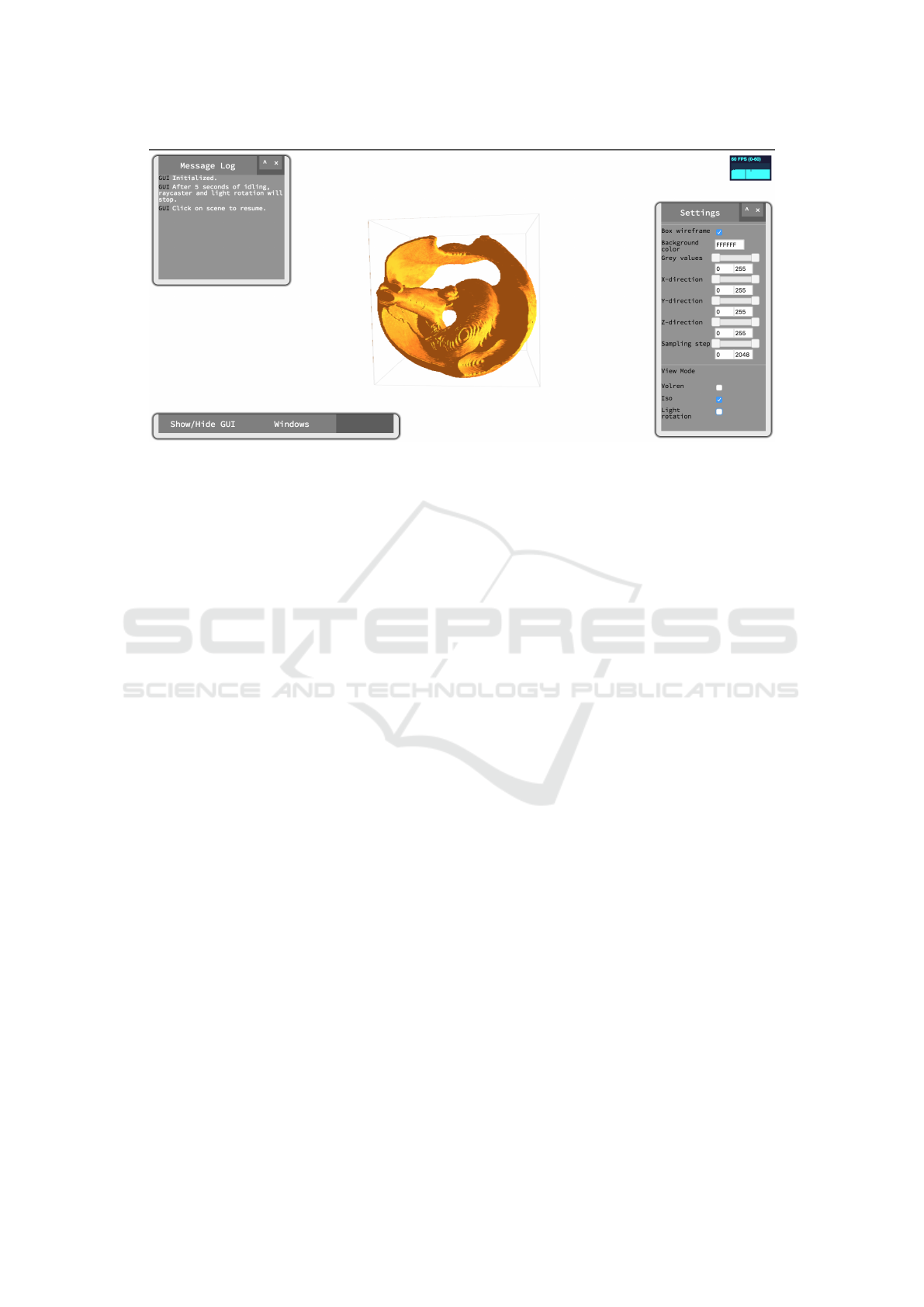
Figure 1: A biological screw found in a bettle’s leg (van de Kamp et al., 2011) rendered by the WAVE client user interface

using the surface rendering method.

slicemaps as caches instead. In order to achieve an

optimal visual quality with reasonable performance,

our framework selects the cache with a suitable level-

of-detail (LOD) by evaluating the visual resolution

and the performance of the client graphical device.

Moreover, the simplicity of the slicemap allows us to

optimize processing tasks between the server and the

client by minimizing data transfers and server loads

for better scalability. The server loads are further al-

leviated as we prepare the reduced data set in advance

using low-priority batch jobs and cache the data either

temporarily or permanently according to the conﬁgu-

ration of the system.

By utilizing both the client and the server re-

sources, the WAVE framework is able to produce an

interactive 3D preview on most client devices with-

out being restricted neither by the data size nor by

the data latency. Our framework supports zoom-on-

demand approach, which reloads the user selected re-

gion using caches with a high level-of-detail. Fur-

ther in this paper, we evaluate our framework using

a data set from the entomology science experiment.

Our framework is open source, and it is generally ap-

plicable to other science domains where an interactive

3D web-based data previewer is required.

2 RELATED WORK

In this section, we present relevant works in large data

processing that helps in visual data browsing. Two

viable approaches to realize our goal are in-situ vi-

sualization and multi-resolution techniques (Childs,

2007).

2.1 in situ Visualization

Rivi et. al. described three different approaches in

in-situ visualization: they are tightly coupled, loosely

coupled, and hybrid approaches. These approaches

are still widely used in many High Performance Clus-

ter (HPC) facilities. There is no single universal tech-

nique for in-situ visualization as each approach can be

beneﬁcial in each different use case (Rivi et al., 2012).

The tightly coupled approach does not require

data movement, with visualization and computation

running on the same nodes or machine. Numer-

ous applications using this approach can be seen in

SciRun (Johnson et al., 1999), Hercule (Tu et al.,

2006), ADIOS and CoDS (Zhang et al., 2012), and

YT package (Turk et al., 2010). However, this

approach requires large investments in visualization

equipments and knowledge in the simulation code.

The loosely coupled approach on the other hand

has separate set of resources involving data move-

ment over the network. For example, data process-

ing is done on the server while images are streamed

to the client. This approach offers ﬂexibility but at

the expense of being restricted by the network band-

width. Applications using such approach can be seen

in Strawman (Larsen et al., 2015), Image-based ap-

proach (Ahrens et al., 2014), Catalyst (Lorendeau

et al., 2013), PreDatA and ADIOS (Malakar et al.,

2010), and EPSN (Esnard et al., 2006).

The hybrid approach is the most similar to the

WAVE framework, in which data is reduced in a

tightly coupled setting and later sent to a concurrent

resource for further post processing. This approach

inherits advantages from the tightly coupled and the

loosely coupled approaches, and at the same time

WAVE: A 3D Online Previewing Framework for Big Data Archives

153

minimizes their drawbacks, e.g. ParaViewWeb (Rivi

et al., 2012), X3DOM (Behr et al., 2009). Here,

web browser can be used as the client resource to

render the data. Due to the advancement in web

technologies that exploits the power of GPU through

WebGL (Khronos, 2011), data can be processed in

parallel even on a less powerful mobile device. Con-

gote et al. presented an early work on web-based vol-

ume visualization using the GPU-based ray marching

approach in WebGL (Congote et al., 2011), which

proved to be an interesting option. Being inspired

by their work, traits of their work can be seen in our

framework, especially the usage of the slicemap as

our main data object.

2.2 Multi-resolution Techniques

Isenberg et. al. presented an analysis regarding re-

cent visualization techniques and categorized multi-

resolution techniques, view-dependent visualization,

and level of detail under the main category abstrac-

tion, simplication, approximation (Isenberg et al.,

2017). These subsets of techniques complement each

other to achieve an efﬁcient rendering at an interactive

rates. Although multi-resolution techniques had been

presented early back in 1983 by Williams (Williams,

1983), such approach is still valid, as the system bot-

tleneck continues to remain at the network bandwidth.

In this section, we discuss on applications that uti-

lized these techniques. Burigat and Chittaro studied

the feasibility of overview-and-demand visualization

on mobile devices (Burigat and Chittaro, 2013). In

their study, they ﬁrstly loaded a map with the coarsest

level of detail, and a map with better level of detail

only on a higher zoom level.

Lu et. al. introduced a ﬂexible LOD con-

trol scheme to effectively explore the ﬂow structures

and characteristics on programmable graphics hard-

ware (Lu et al., 2015). In their control scheme, the

output textures were created according to a sparse

noise model, taking the depth distance of a point and

the corresponding brick contribution into considera-

tion.

Kimball et. al. introduced a level of detail algo-

rithm which enables interactive visualization of mas-

sive, unstructured, particle data sets (Kimball et al.,

2013). They created a multi-resolution pyramid of

volume slabs and stacked them into volumes. Each

slabs vary in level of detail and full resolution slabs

are used at the closest view.

Zinsmaier et. al. proposed a technique that allows

straight-line graph drawings to be rendered interac-

tively with adjustable level of detail (Zinsmaier et al.,

2012). They used the density-based node aggrega-

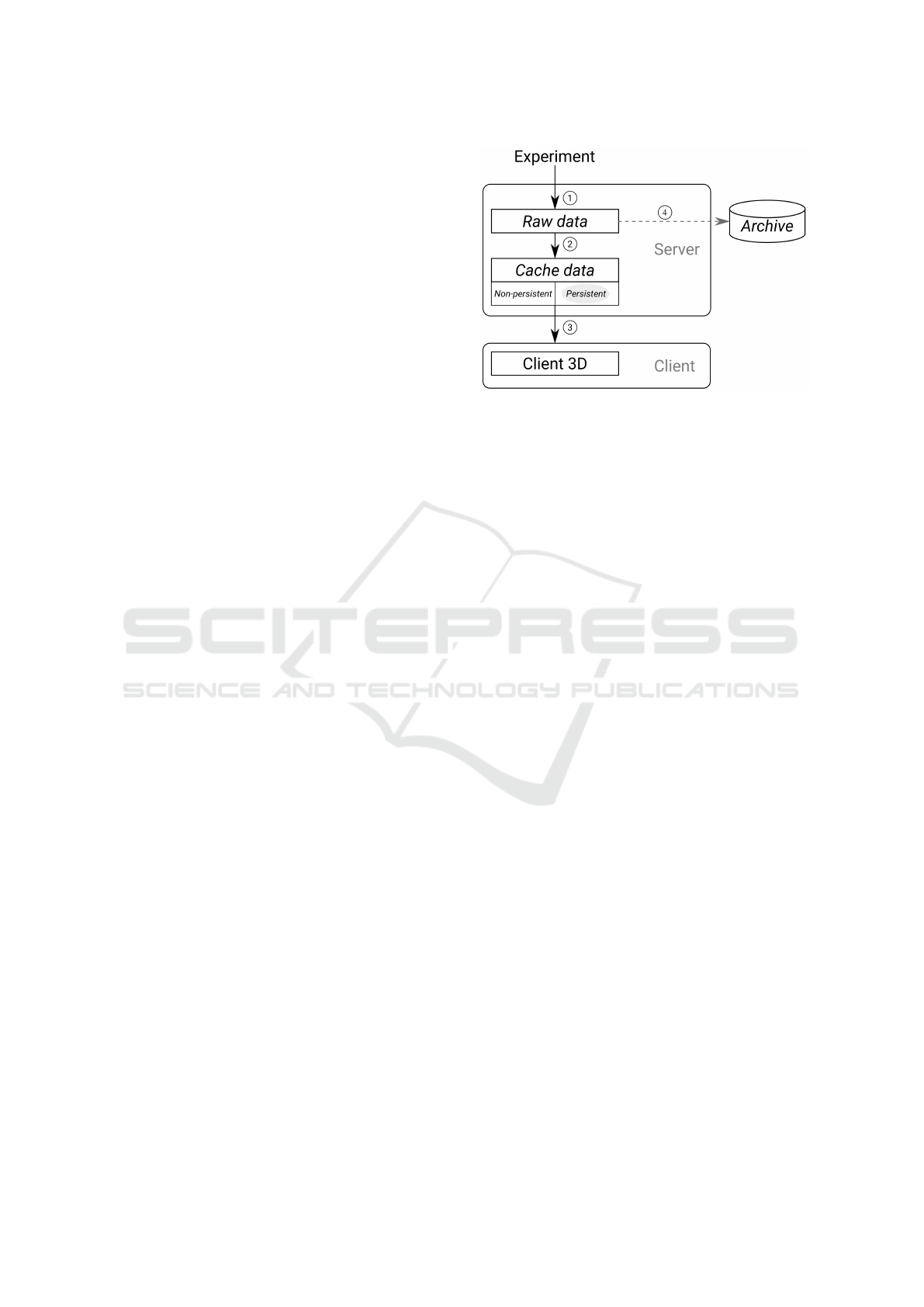
Figure 2: The data ﬂow of the WAVE framework.

tion and the edge aggregation to select visual patterns

at different levels of detail. They were able to show

graphs with up to ∼ 107 nodes and up to ∼ 106 edges

at interactive rates.

All these applications ﬁrst prepared a series of

LOD data governed by its varying visual detail, e.g.

resolution. A control logic was then applied to select

the best LOD data according to the intended visual-

ization. In the WAVE framework, we also prepare a

hierarchy of multi-resolution slicemaps varying in its

image resolution. A cache selection is put into ac-

tion to select the best slicemap according to the client

hardware.

3 THE WAVE FRAMEWORK

An effective large data previewing framework must

address two main challenges: they are large data

processing and interactive scalability across various

client hardware. The large data can be either pro-

cessed in parallel or reduced in size. We use the latter

approach, where our framework mainly processes the

data at the ofﬂine data preprocessing stage, the online

server data preparation stage, and the client visualiza-

tion stage.

As shown in Figure 2, the ofﬂine data preprocess-

ing stage monitors new incoming data from the ex-

periment using a cron service (Step 1) and caches the

LOD data (Step 2). Depending on the client perfor-

mance, our framework selects the best cache data that

provides a good visual quality and a reasonable band-

width transmission (Step 3). The client visualization

stage then render the selected data by performing a

direct volume rendering or a surface rendering. Dur-

ing the online server data preparation stage, a high-

resolution slicemap is generated on-the-ﬂy upon user

demand. The generated slicemap uses the cache data

IVAPP 2017 - International Conference on Information Visualization Theory and Applications

154

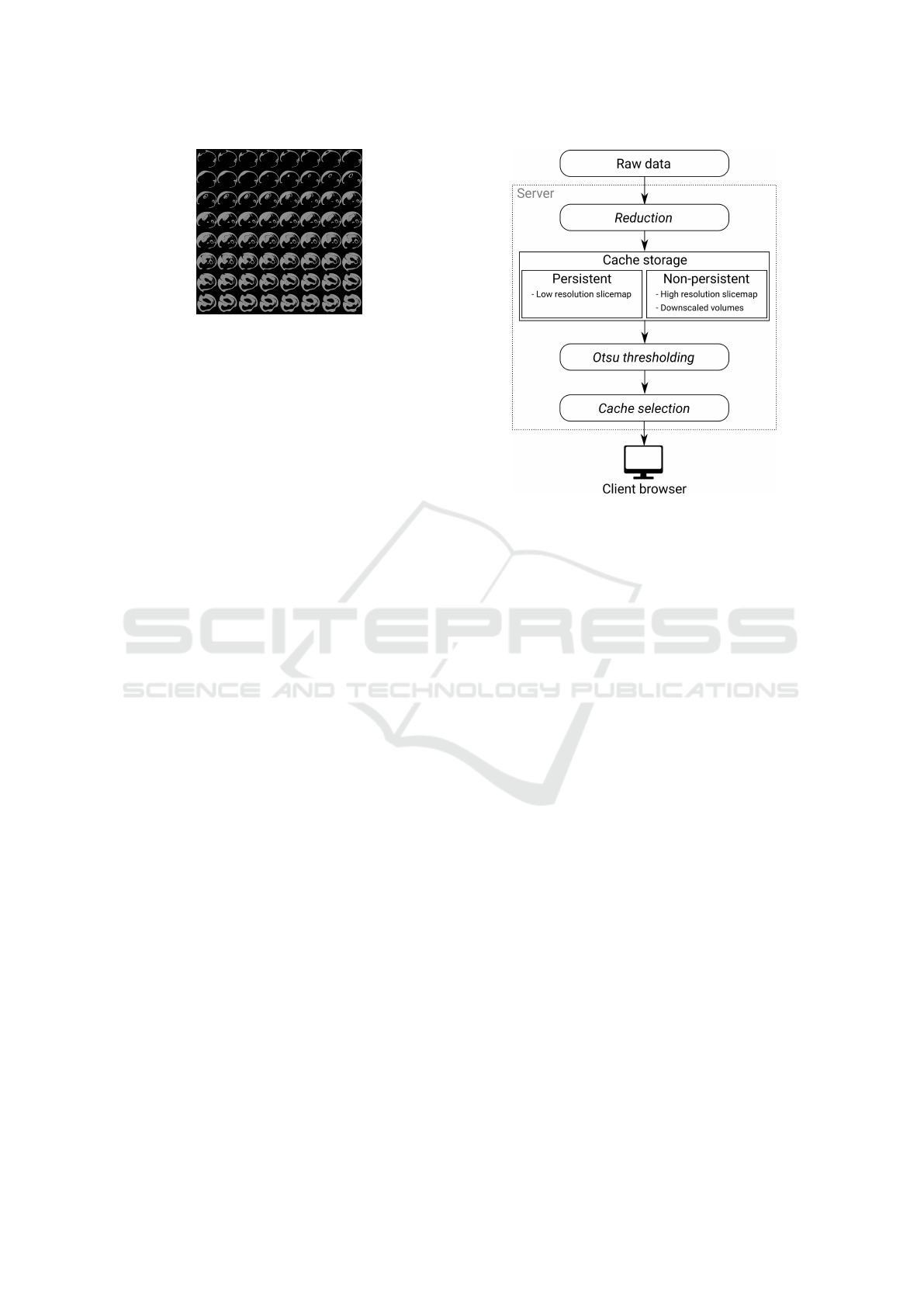
Figure 3: An 8 × 8 slicemap of a biological screw (van de

Kamp et al., 2011).

to reduce the wait time.

To deal with the growing data size in the server

storage, data that are no longer in active use, are

pushed to a dedicated remote archive (Step 4). At

the same time, non-persistent caches are ﬂushed while

preserving persistent caches. These persistent cache

data are later served as a list of visual previews for

remote data browsing.

Throughout our framework, the usage of the

slicemap is motivated by the lack of 3D texture sup-

port in the WebGL. This restriction led us to emulate

the 3D texture by utilizing the available 2D texture

feature. By packing the image slices into mosaic for-

mat (slicemap), we load these slicemaps into the tex-

ture memory and and use the pixel shader to calculate

the x,y coordinate from the z coordinate of the cor-

responding slicemap. For example, a 256 × 256 × 64

volume constitutes a slicemap with 2048 × 2048 pix-

els arranged as an 8 × 8 grid of 256 × 256 pixels im-

age slice. Figure 3 shows an 8 ×8 slicemap generated

from a segmented biological screw data (van de Kamp

et al., 2011).

3.1 Server Architecture

Figure 4 shows the WAVE server architecture, where

each data set undergoes the data reduction, the data

caching, and the data thresholding stages before serv-

ing the slicemap to the client.

Starting from the raw data stage, a cron service

monitors incoming new data sets and triggers a se-

ries of batch jobs. These batch jobs are mainly dis-

cussed in the data reduction stage (Section 3.1.1),

where the data size is reduced and transformed into

cache formats. These formats are categorized as low-

resolution slicemap, high-resolution slicemap, and

downscaled volume. With cache data readily avail-

able, our framework performs progressive loading by

loading a low-resolution slicemap ﬁrst, followed by a

suitable high-resolution slicemap loading in the back-

ground. The suitable high-resolution slicemap in this

context refers to the slicemap that satisﬁes the client

Figure 4: Detailed server architecture.

hardware requirement.

We also allow online generation of slicemap

with level of detail higher than the high-resolution

slicemap in the zoom-on-demand approach (Sec-

tion 3.3). During the online slicemap generation, the

cached downscaled volume is used to minimize the

wait time. Only the low-resolution slicemap is stored

as a persistent cache, whereas the other caches are

non-persistent. While each raw data is stored in a

folder, we store its respective caches within its folder

as well.

3.1.1 Data Reduction

Due to the large data size, we downscaled the raw

data before transforming it into a slicemap. We used

the Lanczos ﬁlter from ImageMagick to perform the

downscaling operation. After downscaling, we trans-

formed the downscaled volumes into a PNG-format

slicemap. For example, a raw data set of a carpen-

ter ant (Garcia et al., 2013) with 2016 × 2016 × 2016

voxels (7.7 GB) can be downscaled and transformed

into a low-resolution slicemap with 256 × 256 × 256

voxels (2 MB). Figure 5 shows the processing time of

each operation during the online server data prepara-

tion performed on a 64 bit Quad-Core Intel(R) Core

i7-3770 CPU at 3.40 GHz. These operations are dis-

cussed more in Section 3.3. Our initial study shows

that the time taken to perform the downscaling op-

eration is much higher than the others, which moti-

vates us to precompute a set of downscaled volumes

as caches. In our framework, we had chosen down-

scaled volumes with 256

voxels, 512

voxels, 768

WAVE: A 3D Online Previewing Framework for Big Data Archives

155

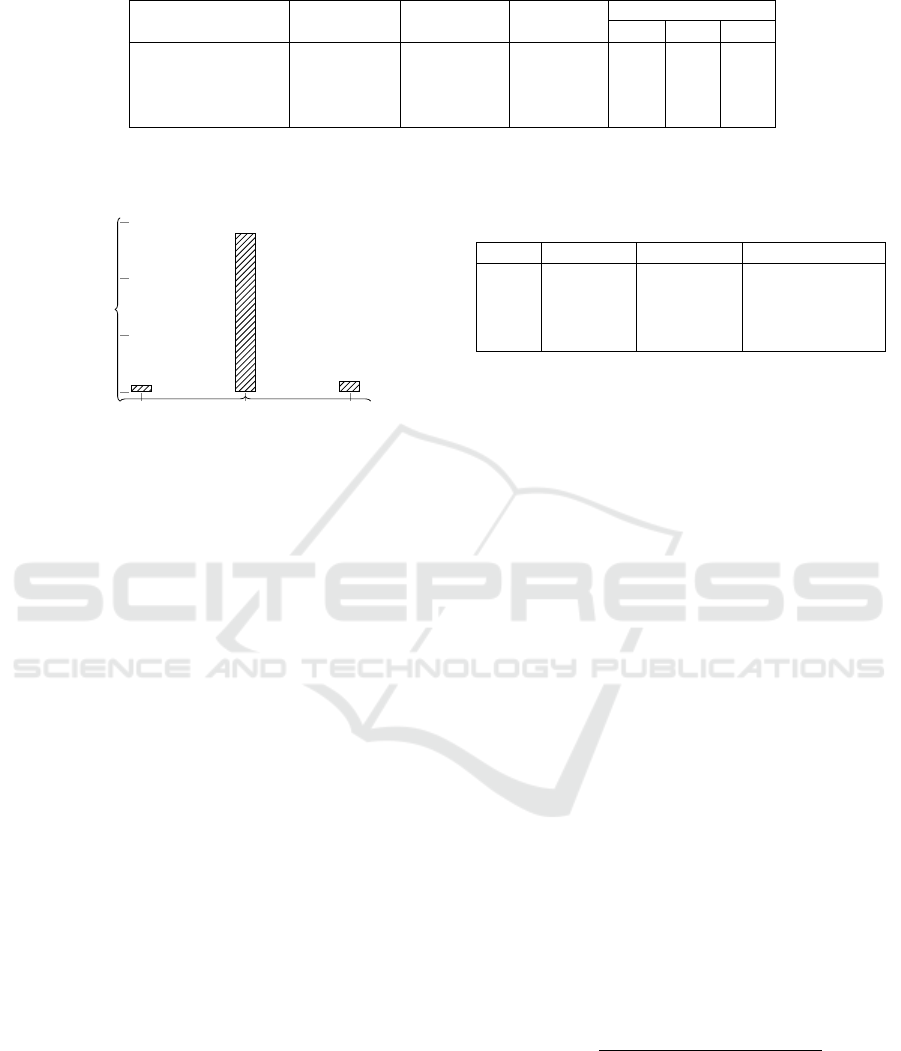
Table 1: Relationship between the varying size of the slicemap and the frame rate of the client devices.

Device (GPU) Texture Unit Texture Size GFXbench

Voxels (fps)

(pixels) (frames) 128

256

512

Desktop (Titan) 32 16384

107898 1301 649 245

Laptop (GT750M) 16 16384

8821 200 112 45

Desktop (HD4000) 16 8192

3362 102 32 11

Phone (Adreno330) 16 4096

1601 30 12

The frame metrics are taken from GFXBench benchmarking suite tested with T-Rex off-screen 1080p (Kishonti, 2011).

This metric shows the performance of each GPU (higher the better).

<15fps. Unacceptable user perception quality (Claypool et al., 2006).

crop

downscale transform

2.08

56.03

3.61

Processing time, s

Figure 5: Online server data preparation of a 2016×2016 ×

2016 voxels carpenter ant data set (Garcia et al., 2013).

voxels, and 1024

voxels. By having slicemaps and

downscaled volumes as caches, our framework is able

to serve data at an interactive rate.

3.1.2 Multi-resolution Support

To support a broad range of clients with varying hard-

ware, multi-resolution slicemaps that vary in resolu-

tion details are created. As the size for slicemaps may

differ according to the client hardware, we performed

a study on the relationship between the varying size of

slicemaps and the frames-per-second of various client

devices. Here, we had chosen a broad range of client

devices, covering from less powerful mobile phone up

to powerful desktop. The performance of each client

device rendering multiple data sizes is shown in Ta-

ble 1. In this study, we assumed that the data size is

inversely proportional to the scale of data transmis-

sion. In other words, a small data size results in a

high data transmission, whereas a larger data size re-

sults in a lower data transmission. Detailed time taken

in data transmission for various slicemap sizes under

different network presets is shown later in Section 4.

We determine the user acceptance metric base on the

study conducted by Claypool et al.. In their study,

the user performance and the user perception quality

dropped signiﬁcantly when the frames-per-second is

below 15fps (Claypool et al., 2006).

As shown in Table 1, the data set with 128

vox-

els provides the best frames-per-second across the se-

lected client devices; data sets with 256

voxels and

512

voxels are imposing problems on the smaller

Table 2: Multi-resolution hierarchy scheme deﬁnition.

Level Scheme Voxels Format

0 256

× 2

16777216 256 × 256 × 256

1 256

× 2

33554432 256 × 256 × 512

2 256

× 2

67108864 512 × 512 × 256

3 256

× 2

134217728 512 × 512 × 512

client device. However, data set with 128

voxels

delivered a visual object that is no longer recogniz-

able leading us to select a slicemap with 256

vox-

els as the low-resolution slicemap, and higher voxel

size as high-resolution slicemaps. Although the data

set with 256

voxels had an unacceptable frames-per-

second (<15fps) on the mobile device, but we can fur-

ther improve the client rendering with an optimized

code. Though it may seem that only two data sizes

are available as cache levels, we vary the z-axis to

give us more granularity for gradual visual improve-

ment. We deﬁne a hierarchy of levels varying in the

amount of voxels. With N levels of slicemaps, each

level N slicemap contains 256

× 2

voxels. In our

framework, we precompute four levels of slicemaps

to cover most client resources (Table 2). Our scheme

can be further extended depending solely on the ad-

vancement of the hardware.

In the cache selection stage, a suitable slicemap

is selected depending on the client hardware re-

quirement. There are two parameters that deter-

mine the client performance: texture size and tex-

ture unit. The texture size deﬁnes the image reso-

lution of the slicemap, whereas the texture unit de-

ﬁnes the amount of slicemaps that can be rendered.

To select the suitable slicemap level, the product of

the texture unit and the texture size of the mobile

device is used as our baseParameter (16 × 4096 =

65536). We then compute the appropriate cache

level by blog

clientTextureUnit×clientTextureSize

baseParameter

c, where

clientTextureUnit and clientTextureSize are acquired

from the client hardware requirements.

3.1.3 Data Thresholding

We are mostly dealing with electron microscopy im-

ages of biological specimens, that are especially noisy

IVAPP 2017 - International Conference on Information Visualization Theory and Applications

156

(a) Grey value: 0 - 255 (b) Grey value: 107 - 255

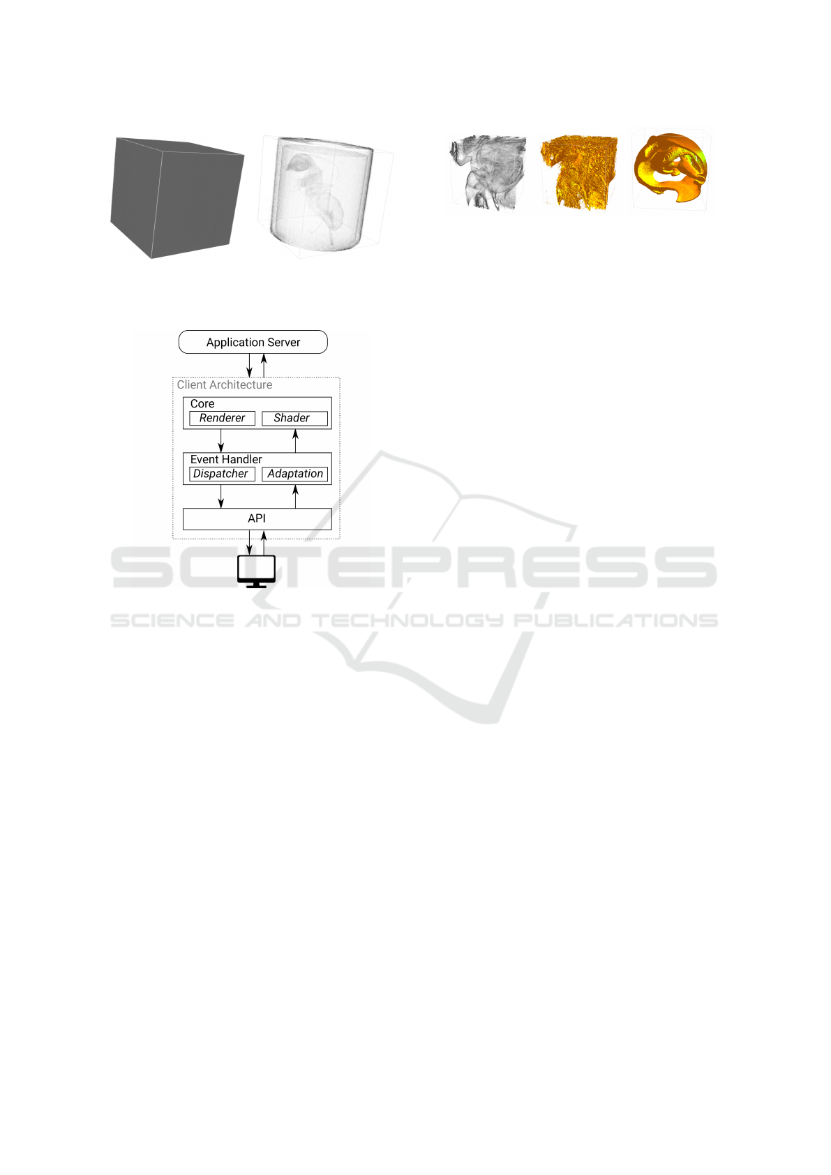
Figure 6: A 3D volume rendering without (a) and with (b)

Otsu thresholdings. The calculated Otsu threshold is 107.

Figure 7: Detailed client architecture.

and low contrasted (Coudray et al., 2010). With no

prior knowledge of the region of interest, our visual

previewer framework might end up showing all avail-

able grey values from the data set, rendering a 3D ob-

ject that ﬁlls up the entire volume as shown in Fig-

ure 6a. Under such circumstances, the user can ﬁlter

out the grey values using the WAVE interface settings

(Figure 1). However, a visual previewer framework

that requires manual thresholding from users is not

easy to use. Instead, we adopt the Otsu thresholding

method on our low-resolution slicemap.

The Otsu thresholding method tries to minimize

the combine spread between the two clusters by mov-

ing the threshold along the grey value range (within-

class variance). We chose another variation of the

Otsu method that depends only on the difference be-

tween the means of the two clusters, thus avoiding

the need to calculate differences between individual

intensities and the cluster means (Morse, 2000). This

variant is described in (1).

Between

(T ) = n

(T )n

(T )[µ

(T ) − µ

(T )]

(1)

where T is the varying threshold along the range

of grey values. σ

Between

is the mean difference be-

tween the two clusters. n

(T ) is the sum of pixels in

(a) (b) (c)

Figure 8: A 3D visualization of segmented and non-

segmented biological screw data sets using the volume ren-

dering and the surface rendering methods. (a) Volume ren-

dering with raw data set. (b) Surface rendering with raw

data set. (c) Surface rendering with segmented data set.

the background (below threshold). n

(T ) is the sum

of pixels in the foreground (above threshold). µ

(T )

and µ

(T ) are variances of pixels in background (be-

low threshold) and foreground (above threshold), re-

spectively. We select the threshold that gives us the

highest mean difference between the two clusters.

Although one might argue that the Otsu thresh-

olding method should be performed on the raw data.

But, we achieved great success performing the Otsu

method on the low-resolution slicemap, in which the

correct threshold value is acquired in a much shorter

time. This threshold value can be applied to all other

slicemaps stemming from the same raw data. Fig-

ure 6b shows a 3D object rendered with an Otsu

threshold of 107. It is worth noting that the thresh-

old value serves as a reference for the minimum grey

value, and user still has the option to change the

threshold value through the WAVE user interface.

3.2 Client Architecture

Our WAVE client is implemented in Javascript, which

is written on top of the ThreeJS library (Cabello,

2011) that utilizes WebGL (Khronos, 2011). The

Javascript language offers platform independence,

and it can be interpreted at every major client browser.

Figure 7 depicts our client architecture, which is

consist of a core layer, an event handler layer, and

an application programming interface (API) layer.

The core layer is responsible for rendering the

slicemap. Within the core layer, the renderer and the

shader components perform the direct volume ren-

dering based on the work from Kruger and Wester-

mann (Kruger and Westermann, 2003) and the lo-

cal surface illumination model using the Blinn-Phong

model (Blinn, 1977). Figure 8 shows 3D visualiza-

tions of both raw and segmented biological screw data

sets in both volume rendering and surface rendering

modes. Although we support both the volume ren-

dering and the surface rendering methods, the volume

rendering method is more suited to visualize new data

set due to its ability to inspect the inner structure; The

surface rendering method provides an attractive visual

WAVE: A 3D Online Previewing Framework for Big Data Archives

157

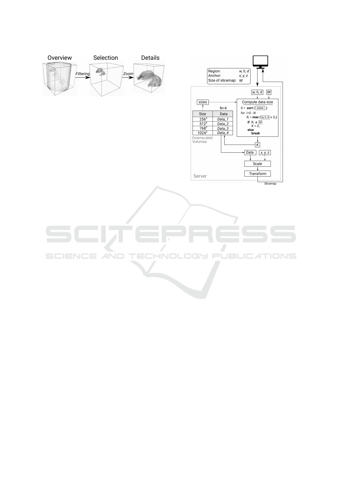
Figure 9: An illustration of zoom-on-demand feature.

quality on the segmented data set (Figure 8c).

In the volume rendering approach, ray is emulated

and sampled with a constant step size. These sampled

points then contribute to the ﬁnal composition func-

tion. By varying the step size, the performance and

visual detail of the rendered object can be adapted ac-

cordingly. This is a matter of trade off between per-

formance and visual detail, where large step size leads

to faster rendering but less visual details. We reduce

the step size during a dynamic 3D object movement

and increase the step size when the object is static.

In order to facilitate user interactions from the

browser, the WAVE client provides a set of API.

These API calls allow the user to conﬁgure the core

layer from the browser directly. Furthermore, they

provide an easy integration into a variety of web

applications with varying designs and layouts, e.g.

Biomedisa web application (Lösel and Heuveline,

2016). In the event handler layer, the adaptation com-

ponent and the dispatcher component handle the user

state and the core layer state between the WAVE client

and the user interface. In particular, our client frame-

work provides four features to inspect and analyze the

data set: (a) by selecting the grey value threshold, (b)

by adjusting the transfer function, (c) by changing the

camera position and (d) by slicing through the 3D ob-

ject. The ﬁrst feature (a) is useful to inspect a new

data set, where the grey value threshold is selected

to remove the unwanted background. The second fea-

ture (b) enables transfer function update (Pﬁster et al.,

2001); Each grey value is assigned a colour according

to the selected function to help in classiﬁcation of the

data set. The third feature (c) changes the camera po-

sition of the viewer in the 3D scene allowing the user

to view the 3D data in any angle and distance. The

last feature (d) slices through the 3D object in x, y

and z-directions providing ﬂexibility for the user to

inspect the inner structure of the data set.

3.3 Zoom on Demand

The WAVE framework supports the zoom-on-demand

approach, which follows the visual information seek-

ing mantra, overview ﬁrst, zoom and ﬁlter, then

details-on-demand (Shneiderman, 1996). The zoom-

on-demand approach allows the user to select a re-

Figure 10: Selection of the cached downscaled volumes ac-

cording to client requirements.

gion of interest from the 3D volume for more details

(Figure 9). Using the browser cache (high-resolution

slicemap), a new slicemap is initally generated con-

sisting of the selected region, where the number of

slices is determined and each image slice is cropped

accordingly. These operations are performed locally

in the client browser using the JavaScript language.

At the same time, another slicemap with higher de-

tails containing the selected region is created from

the server (online server data preparation). The on-

line server data preparation uses the readily cached

downscaled volume for fast slicemap generation.

To select the downscaled volume, the intended

slicemap size, M, the selected region parameters,

[w, h, d], and the anchor points, [x, y, z], are acquired

from the client, where x, y, z are the starting points of

the selected region; and w, h, d are the width, height

and depth of the selected region (x, y, z, w, h, d ∈

[0, 1]). Figure 10 shows the process to select the suit-

able downscaled volume. To compute the suitable

downscaled volume size, we iterate through all the

sizes from 256 to 1024. At each iteration, we select

the product of the region parameters, [w, h, d], and the

current iterated size, S

, that is less than the size of the

intended slicemap, M. Whenever the current iterated

size, S

, is larger than the intended size, M, the previ-

ous iterated size is selected. The selected downscaled

volume is then scaled according to the region param-

eters and the anchor points. Lastly, the scaled data is

transformed into the intended slicemap format before

serving it back to the client.

IVAPP 2017 - International Conference on Information Visualization Theory and Applications

158

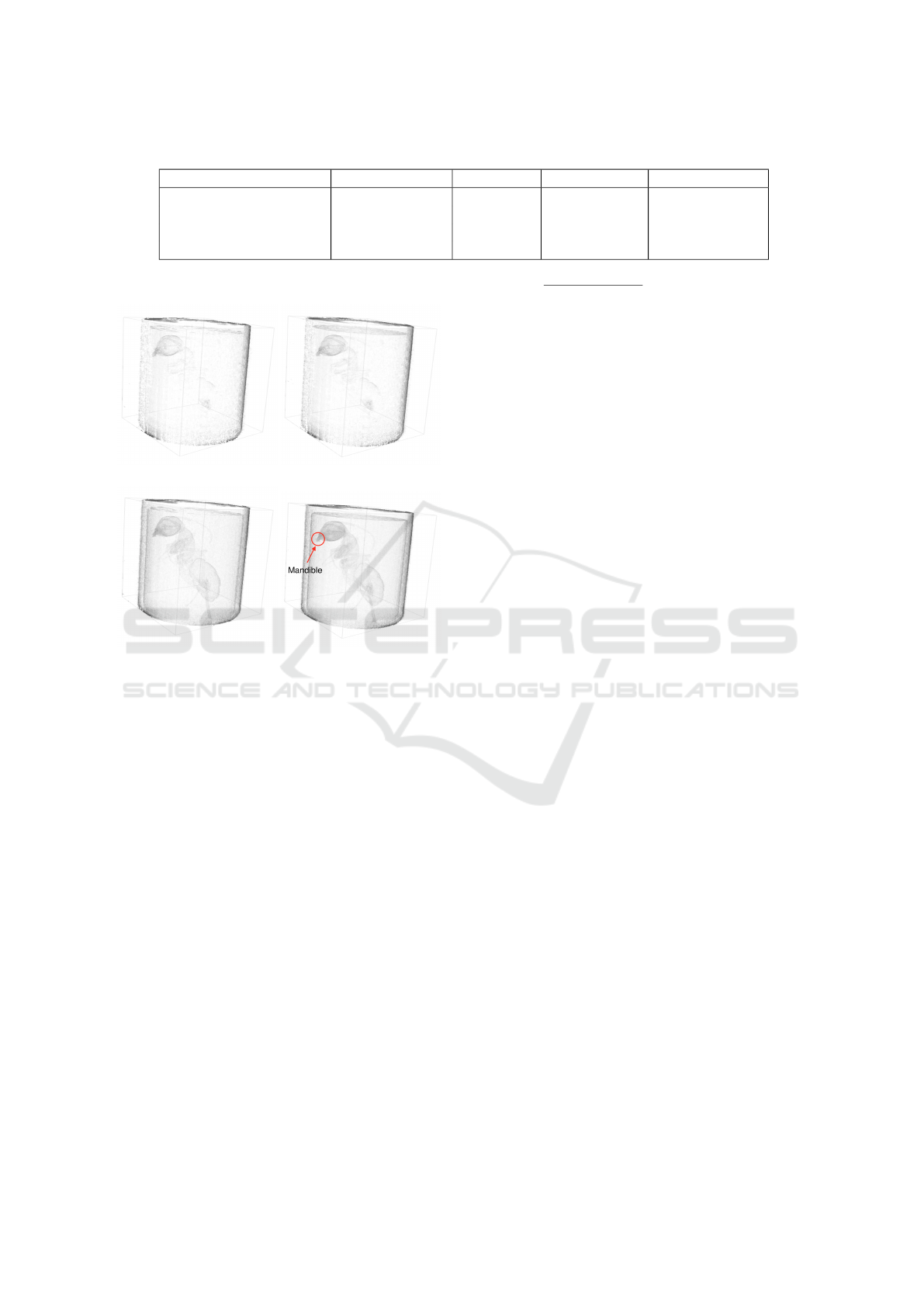
Table 3: A series of slicemaps produced from the carpenter ant data set (Garcia et al., 2013) in the WAVE server.

Category Scheme Voxels Slicemap Size Reduction Ratio

Low-resolution (level 0) 256 × 256 × 256 16777216 1.90 MB 488

High-resolution (level 1) 256 × 256 × 512 33554432 3.90 MB 244

High-resolution (level 2) 512 × 512 × 256 67108864 9.70 MB 122

High-resolution (level 3) 512 × 512 × 512 134217728 20.10 MB 61

Reduction ratio is used to quantify the reduction in data representation size (voxels) produced from the WAVE server. The

raw data set consisted of 2016 ×2016 ×2016 voxels. ReductionRatio =

rawAmountVoxels

reducedAmountVoxels

(a) 256 ×256 ×256 (level 0) (b) 256 ×256× 512 (level 1)

Figure 11: Four 3D objects of a carpenter ant (Garcia et al.,

2013) rendered from our multi-resolution slicemaps: (a)

AE: 0, RMSE: 0%, base image, (b) AE: 90264, RMSE:

0.049%, (c) AE: 178678, RMSE: 0.060%, and (d) AE:

201959, RMSE: 0.068%.

4 EVALUATION

The WAVE framework is currently implemented in

the Astor web portal (Astor, 2014), in the USCT

application (Ruiter et al., 2013) and also in the

Biomedisa online segmentation application (Lösel

and Heuveline, 2016). To illustrate the image quality

and the performance delivered by our framework, we

selected a carpenter ant data set (Garcia et al., 2013)

with 2016

voxels. The carpenter ant belongs to the

order of Hymenoptera under the family of Formici-

dae. This raw data was transformed into a series of

slicemaps according to our multi-resolution scheme

deﬁnition (Table 3). A set of downscaled volumes

were also cached in the server. Throughout our evalu-

ation, we used a 64 bit Quad-Core Intel(R) Core i7-

3770 CPU at 3.40 GHz as our server, and a Mac-

bookPro running on a NVIDIA GeForce GT750M as

our client.

4.1 Visual Quality

Serving as a large data previewing framework, our

framework must be able to present a recognizable

visual object using our hierarchy of multi-resolution

slicemaps. Also, the zoom-on-demand approach must

provide more details on the selected sub-region.

The visual quality of the WAVE framework is de-

termined according to the amount of pixels rendered

on the browser screen. More pixels imply that more

details are rendered, thus giving us a better preview.

We used the absolute error count metric (AE) to show

the number of different pixels in a masked image. The

mask image refers to a resultant image from mask-

ing the test image against a base image. Also, we

used the root mean squared error (RMSE) to show

the gradual visual improvement in our framework ap-

proaches. We performed these widely used image

quality metrics on 3D object screenshots rendered

by multi-resolution slicemaps and zoom-on-demand

slicemaps.

Figure 11 shows previews of the carpenter ant

rendered by our multi-resolution slicemaps, from

level 0 to level 3. Here, the low-resolution slicemap,

level 0, was selected as the base image tested against

four multi-resolution slicemaps. Although the low-

resolution slicemap (level 0) has lesser details, the

structure still resembles the carpenter ant. The

mandible of the carpenter ant is visible in all rendered

objects. Nevertheless, we can see a gradual visual im-

provement from level 0 to level 3. The gradual vi-

sual improvement is also indicated from the increas-

ing value of AE and RMSE.

We further evaluated the zoom-on-demand ap-

proach, in which 3D object with higher details are

created from browser cached slicemap and later

from server cached downscaled volume. Figure 12

shows the upper body of the carpenter ant rendered

from browser cached multi-resolution slicemaps from

level 0 to level 3. Although the level 2 slicemap ob-

ject had a higher AE and RMSE values than the level

3 slicemap object, the smooth edges in the level 3

slicemap object lent itself to a lesser masked region,

WAVE: A 3D Online Previewing Framework for Big Data Archives

159

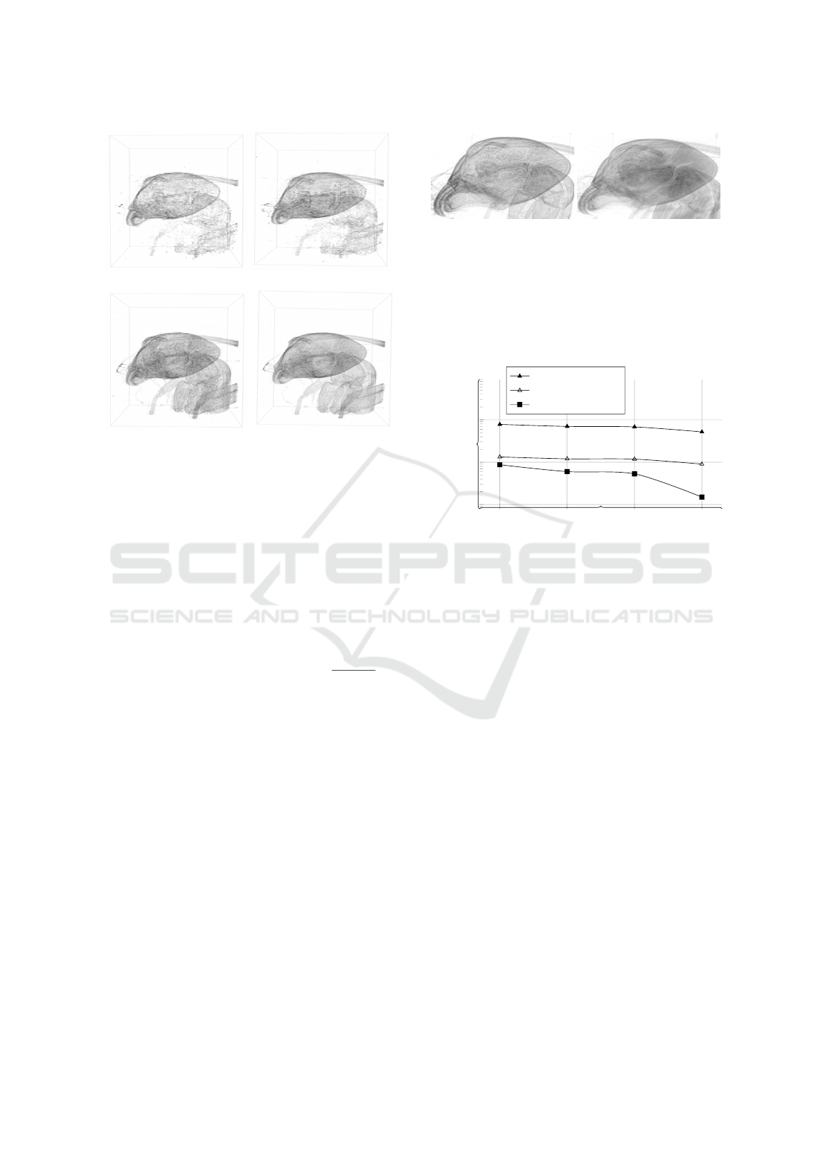
(a) level 0 (b) level 1

Figure 12: The visual quality of the zoomed carpenter ant

(upper body) created by multi-resolution slicemaps in the

client browser using the JavaScript language: (a) AE: 0,

RMSE: 0%, base image, (b) AE: 126586, RMSE: 0.055%,

RMSE: 0.069%.

thus resulting in a slightly smaller AE and RMSE val-

ues.

During the zoom-on-demand, our framework trig-

gered a request to the server for a slicemap with better

quality. In this particular test, our client was running

on a GTX Titan graphic card with a texture unit and

texture size of 32 and 16384px, respectively. Thus, the

cache level suitable for our client is blog

32×16384

65536

c =

3. The level 3 slicemap consists of 512 × 512 × 512

voxels, resulting in M value of 134217728. We se-

lected the zoom region (carpenter ant’s head) using

the WAVE user interface and sent [x, y, z, w, h, d] =

[0.15, 0.43, 0.62, 0.38, 0.38, 0.38] to the server. Base

on the selection algorithm shown in Figure 10, the

downscaled volume of size 1024

was selected. Fig-

ure 13 compares the visual quality of 3D objects ren-

dered from the browser cached and the server cached

slicemaps using the same set of parameters.

The results showed that the WAVE framework

is capable of delivering recognizable visual pre-

views from the large data using the prepared multi-

resolution slicemaps. Even the 3D objects rendered

by the newly generated slicemaps from the browser

cached slicemap and the server cached downscaled

volume are able to provide more visual details for fur-

ther analysis.

(a) Browser cached (level 3

slicemap).

(b) Server cached (Down-

scaled volume 1024

Figure 13: A comparison between a browser cached (level 3

slicemap) and a server cached (Downscaled volume 1024

)

on a client (GTX Titan) with M = 512 × 512 × 512 and

[x, y, z, w, h, d] = [0.15, 0.43, 0.62, 0.38, 0.38, 0.38]. The se-

lected region is the carpenter ant’s head. (a) RMSE: 0.24%,

(b) RMSE: 0.29%. A white image is used as the base image

to perform image quality comparison.

Level 0 Level 1 Level 2 Level 3

100

1,000

frames-per-second, fps

GTX Titan (1301

)

GT750M (200

)

HD4000 (102

)

Figure 14: The frames-per-second for multi-resolution

slicemaps on various client resources (sampling step=256).

refers to the frame metrics from the WAVE framework

tested against each client hardware with a test data size of

128

voxels (the higher the better).

4.2 Performance

The WAVE performance is determined mainly by the

user experience, which is related to the system in-

teractivity and latency. The ﬁrst tests measure the

responsiveness of the client-side rendering; this rep-

resents average frame rates across various client de-

vices. However, frame rate alone does not give us

an overview of the overall performance. The latency

between server-client interaction also affects the per-

ceived system interactivity. Hence, we performed

tests to measure the page load time for various data

sizes, and to measure the total time taken to perform

the online server data preparation (zoom-on-demand).

4.2.1 Frame Rates

The rendering performance of the client hardware is

related to the slicemap size, the volume rendering

sampling step size, and the GPU hardware.

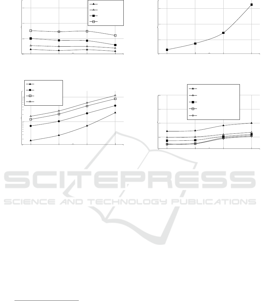
Figure 14 shows the frame rate of our multi-

resolution slicemaps rendered on various client hard-

ware. From the result shown, the slicemap containing

IVAPP 2017 - International Conference on Information Visualization Theory and Applications

160

Level 0 Level 1 Level 2 Level 3

200

400

600

frames-per-second, fps

Steps=1024

Steps=512

Steps=256

Steps=128

Figure 15: The frames-per-second for various slicemaps by

varying sampling steps in MacbookPro (GT750M).

Level 0 Level 1 Level 2 Level 3

100

Page load time, s

Wiﬁ 30 Mb/s

4G 4 Mb/s

DSL 2 Mb/s

3G 1.5 Mb/s

Figure 16: Latency for multi-resolution slicemaps on differ-

ent network presets.

higher details requires better client hardware for bet-

ter performance. We also showed the relationship be-

tween varying sampling step size and the frame rate

on a MacbookPro running on a NVIDIA GeForce

GT750M (Figure 15). This test is only valid for

the volume rendering mode, as the surface rendering

mode stops at the ﬁrst ray intersection point.

4.2.2 Latency

Figure 16 shows the data latency between the server

and the client serving multi-resolution slicemaps un-

der different network presets. Although our frame-

work offers a hierarchy of slicemaps to ensure inter-

active response across a broad range of clients, the

higher slicemap levels require a good network con-

nection to be effective.

According to the client hardware,

a high-resolution slicemap selected by

blog

clientTextureUnit×clientTextureSize

baseParameter

c is loaded.

By zooming onto the upper body of the carpenter ant

([x, y, z, w, h, d] = [0.15, 0.43, 0.62, 0.38, 0.38, 0.38]),

our framework ﬁrst creates a new slicemap from

the browser cached high-resolution slicemap. Fig-

ure 17 shows each slicemap generation time from its

browser cached high-resolution slicemap. Then, our

client requested for a slicemap with higher details

from the server. In practice, our framework selects

the best downscaled volume based on the selection

Level 0 Level 1 Level 2 Level 3

Processing time, s

Figure 17: Performing zoom-on-demand on the client-

side (Javascript) using the browser cached high-resolution

slicemap.

Level 0 Level 1 Level 2 Level 3

100

200

300

400

Processing time, s

Raw (2016

)

Downscaled (1024

)

Downscaled (768

)

Downscaled (512

)

Downscaled (256

)

Figure 18: The data latency in performing the online server

data preparation from server cached downscaled volumes.

algorithm in Figure 10. However, we showed the

processing latency of the online server data prepara-

tion from the raw data and all available downscaled

volumes: 256

, 512

, 768

, and 1024

(Figure 18).

The result showed an improvement of approximately

50 seconds by using the downscaled volume cache

in contrary to creating the slicemap directly from

the raw data. However, there is not much difference

(∼ 3 seconds) in performance between using the

downscaled volume of 256

or the downscaled

volume of 512

The results so far showed the importance of ﬁrst

loading the low-resolution slicemap (level 0) that has

a much lower latency across various network pre-

sets and renders much faster on various client hard-

ware. We also showed the beneﬁt of using the browser

cached slicemap to create the new zoomed slicemap,

while a better slicemap was being created using the

downscaled volume (server cache).

5 CONCLUSIONS AND FUTURE

WORK

We have presented a 3D visual previewing frame-

work for big data archives that promotes data avail-

ability across various clients. The WAVE framework

WAVE: A 3D Online Previewing Framework for Big Data Archives

161

supports the volume rendering and surface render-

ing, which are useful in identifying a new data or a

postprocessed data. Moreover, our framework allows

zoom-on-demand where user can reload a selected re-

gion with higher visual details. To support the diverse

client hardware, we introduced a hierarchy of multi-

resolution slicemaps mainly for the progressive load-

ing approach, in which the low-resolution slicemap

is displayed ﬁrst while a suitable high-resolution

slicemap is loading in the background. By perform-

ing the ofﬂine data preprocessing at the server side,

the framework can provide previews on large data set

at an interactive rate. The ofﬂine data preprocessing

is responsible in reducing the large data size and pre-

pares a series of cache data. These cache data are es-

sential to perform the progressive loading and the on-

line server data preparation (zoom-on-demand). The

visual results and performances of the WAVE frame-

work were promising, which strongly suggested the

WAVE framework being an effective visual previewer

framework.

In future work, we plan to support interactive la-

beling and commenting directly on the biology ob-

ject via our user interface, steering our framework

into becoming a distributed synchronous collabora-

tion tool (Isenberg et al., 2011). We also would like to

introduce new rendering schemes that open up more

visualization opportunities for better data inspection

and analysis. One of the highlights in our work is the

usage of slicemap as our main data object. We could

simplify the in-situ visualization approach by produc-

ing multiple intermediate slicemaps to monitor the

progress of a simulation or segmentation process. As

our slicemap is in an image format, we would further

improve the image compression technique for better

data latency over the network, e.g. compressing im-

age slices into a video. Although the Otsu threshold-

ing method performed seemingly well in our frame-

work, extending the spectrum of thresholding meth-

ods is by all means beneﬁcial (Rosin, 2001; Coudray

et al., 2010). Furthermore, an automated heuristic is

an attractive addition to the WAVE framework, which

selects a rendering method and settings based on the

server performance, the network bandwidth, the client

hardware and the user needs.

ACKNOWLEDGMENTS

The authors would like to acknowledge Fe-

lix Schultze, Alexey Tukalo, Guven Gokdemir

and Wu Chengzhi for their contributions to the

WAVE framework. We also thank Michael Heethoff,

Sebastian Schmelzle, Thomas van de Kamp, Nicole

Ruiter and Torsten Hopp for helpful discussions on

their experiment data sets.

REFERENCES

Ahrens, J., Jourdain, S., O’Leary, P., Patchett, J., Rogers,

D. H., and Petersen, M. (2014). An image-based ap-

proach to extreme scale in situ visualization and anal-

ysis. In Proceedings of the International Conference

for High Performance Computing, Networking, Stor-

age and Analysis, pages 424–434. IEEE Press.

Astor (2014). Astor web portal. https://anka-astor-

portal.anka.kit.edu/.

Behr, J., Eschler, P., Jung, Y., and Zöllner, M. (2009).

X3dom: a dom-based html5/x3d integration model.

In Proceedings of the 14th International Conference

on 3D Web Technology, pages 127–135. ACM.

Blinn, J. F. (1977). Models of light reﬂection for computer

synthesized pictures. In ACM SIGGRAPH Computer

Graphics, volume 11, pages 192–198. ACM.

Burigat, S. and Chittaro, L. (2013). On the effectiveness

of overview+ detail visualization on mobile devices.

Personal and ubiquitous computing, 17(2):371–385.

Cabello, R. (2011). Threejs. https://threejs.org/.

Childs, H. (2007). Architectural challenges and solutions

for petascale postprocessing. In Journal of Physics:

Conference Series, volume 78, page 012012. IOP Pub-

lishing.

Claypool, M., Claypool, K., and Damaa, F. (2006). The ef-

fects of frame rate and resolution on users playing ﬁrst

person shooter games. In Electronic Imaging 2006,

pages 607101–607101. International Society for Op-

tics and Photonics.

Congote, J., Segura, A., Kabongo, L., Moreno, A., Posada,

J., and Ruiz, O. (2011). Interactive visualization of

volumetric data with webgl in real-time. In Proceed-

ings of the 16th International Conference on 3D Web

Technology, pages 137–146. ACM.

Coudray, N., Buessler, J.-L., and Urban, J.-P. (2010). A ro-

bust thresholding algorithm for unimodal image his-

tograms. Pattern Recognition Letters, (31):1010–

1019.

Esnard, A., Richart, N., and Coulaud, O. (2006). A steer-

ing environment for online parallel visualization of

legacy parallel simulations. In 2006 Tenth IEEE In-

ternational Symposium on Distributed Simulation and

Real-Time Applications, pages 7–14. IEEE.

Garcia, F. H., Wiesel, E., and Fischer, G. (2013). The ants

of kenya (hymenoptera: Formicidae)-faunal overview,

ﬁrst species checklist, bibliography, accounts for all

genera, and discussion on taxonomy and zoogeog-

raphy. Journal of East African Natural History,

101(2):127–222.

Isenberg, P., Elmqvist, N., Scholtz, J., Cernea, D., Ma, K.-

L., and Hagen, H. (2011). Collaborative visualization:

deﬁnition, challenges, and research agenda. Informa-

tion Visualization, 10(4):310–326.

Isenberg, P., Isenberg, T., Sedlmair, M., Chen, J., and

Möller, T. (2017). Visualization as seen through its

IVAPP 2017 - International Conference on Information Visualization Theory and Applications

162

research paper keywords. IEEE Transactions on Visu-

alization and Computer Graphics, 23(1).

Johnson, C., Parker, S. G., Hansen, C., Kindlmann, G. L.,

and Livnat, Y. (1999). Interactive simulation and vi-

sualization. Computer, 32(12):59–65.

Khronos (2011). WebGL - OpenGL ES 2.0 for the Web,

https://www.khronos.org/webgl/.

Kimball, J., Duchaineau, M., and Kuester, F. (2013). Inter-

active visualization of large scale atomistic and cos-

mological particle simulations. In Aerospace Confer-

ence, 2013 IEEE, pages 1–9. IEEE.

Kishonti (2011). Gfxbench 4.0. https://gfxbench.com/.

Kruger, J. and Westermann, R. (2003). Acceleration tech-

niques for gpu-based volume rendering. In Proceed-

ings of the 14th IEEE Visualization 2003 (VIS’03),

page 38. IEEE Computer Society.

Larsen, M., Brugger, E., Childs, H., Eliot, J., Grifﬁn,

K., and Harrison, C. (2015). Strawman: A batch

in situ visualization and analysis infrastructure for

multi-physics simulation codes. In Proceedings of the

First Workshop on In Situ Infrastructures for Enabling

Extreme-Scale Analysis and Visualization, pages 30–

35. ACM.

Lorendeau, B., Fournier, Y., and Ribes, A. (2013). In-situ

visualization in ﬂuid mechanics using catalyst: A case

study for code saturne. In LDAV, pages 53–57.

Lösel, P. and Heuveline, V. (2016). Enhancing a diffusion

algorithm for 4d image segmentation using local in-

formation. In SPIE Medical Imaging, pages 97842L–

97842L. International Society for Optics and Photon-

ics.

Lu, D., Zhu, D., Wang, Z., and Gao, J. (2015). Efﬁ-

cient level of detail for texture-based ﬂow visualiza-

tion. Computer Animation and Virtual Worlds.

Ma, K. L. (2009). In situ visualization at extreme

scale: Challenges and opportunities. IEEE Computer

Graphics and Applications, 29(6):14–19.

Malakar, P., Natarajan, V., and Vadhiyar, S. S. (2010).

An adaptive framework for simulation and online re-

mote visualization of critical climate applications in

resource-constrained environments. In Proceedings

of the 2010 ACM/IEEE International Conference for

High Performance Computing, Networking, Storage

and Analysis, pages 1–11. IEEE Computer Society.

Morse, B. S. (2000). Lecture 4: Thresholding. Brigham

Young University.

Pﬁster, H., Lorensen, B., Bajaj, C., Kindlmann, G.,

Schroeder, W., Avila, L. S., Raghu, K., Machiraju,

R., and Lee, J. (2001). The transfer function bake-

off. IEEE Computer Graphics and Applications,

21(3):16–22.

Ressmann, D., Mexner, W., Vondrous, A., Kopmann, A.,

and Mauch, V. (2014). Data management at the syn-

chrotron radiation facility anka. In 10th International

Workshop on Personal Computers and Particle Accel-

erator Controls, PCaPAC 2014.

Rivi, M., Calori, L., Muscianisi, G., and Slavnic, V. (2012).

In-situ visualization: State-of-the-art and some use

cases. PRACE White Paper; PRACE: Brussels, Bel-

gium.

Rosin, P. L. (2001). Unimodal thresholding. Pattern recog-

nition, 34(11):2083–2096.

Ruiter, N., Zapf, M., Dapp, R., Hopp, T., Kaiser, W.,

and Gemmeke, H. (2013). First results of a clini-

cal study with 3d ultrasound computer tomography.

In 2013 IEEE International Ultrasonics Symposium

(IUS), pages 651–654. IEEE.

Shneiderman, B. (1996). The eyes have it: A task by data

type taxonomy for information visualizations. In Vi-

sual Languages, 1996. Proceedings., IEEE Sympo-

sium on, pages 336–343. IEEE.

Szalay, A. and Gray, J. (2006). 2020 computing: Science in

an exponential world. Nature, 440(7083):413–414.

Tu, T., Yu, H., Ramirez-Guzman, L., Bielak, J., Ghattas, O.,

Ma, K.-L., and O’hallaron, D. R. (2006). From mesh

generation to scientiﬁc visualization: An end-to-end

approach to parallel supercomputing. In Proceedings

of the 2006 ACM/IEEE conference on Supercomput-

ing, page 91. ACM.

Turk, M. J., Smith, B. D., Oishi, J. S., Skory, S., Skillman,

S. W., Abel, T., and Norman, M. L. (2010). yt: A

multi-code analysis toolkit for astrophysical simula-

tion data. The Astrophysical Journal Supplement Se-

ries, 192(1):9.

van de Kamp, T., Vagovi

c, P., Baumbach, T., and Riedel, A.

(2011). A biological screw in a beetle’s leg. Science,

333(6038):52–52.

Williams, L. (1983). Pyramidal parametrics. In ACM Sig-

graph Computer Graphics, volume 17, pages 1–11.

ACM.

Zhang, F., Lasluisa, S., Jin, T., Rodero, I., Bui, H., and

Parashar, M. (2012). In-situ feature-based objects

tracking for large-scale scientiﬁc simulations. In High

Performance Computing, Networking, Storage and

Analysis (SCC), 2012 SC Companion:, pages 736–

740. IEEE.

Zinsmaier, M., Brandes, U., Deussen, O., and Strobelt, H.

(2012). Interactive level-of-detail rendering of large

graphs. IEEE Transactions on Visualization and Com-

puter Graphics, 18(12):2486–2495.

WAVE: A 3D Online Previewing Framework for Big Data Archives

163