
An Approach to Evaluate the Impact on Travel Time of Bus Network
Changes
Kathrin Rodríguez Llanes
1
, Marco A. Casanova
1
, Hélio Lopes
1
and José Antonio F. de Macedo
2
1
Department of Informatics, Pontifical Catholic University of Rio de Janeiro, RJ, Brazil
2
Department of Computing, Federal University of Ceará, CE, Brazil
Keywords: Travel Time Estimation, Trajectory Data Mining, Bus Network.
Abstract: This paper proposes an approach to evaluate the impact of bus network changes on bus travel time. The
approach relies on data obtained from buses equipped with GPS devices, which act as mobile traffic sensors.
It involves three main steps: (1) analysis of the bus network to determine which road segments are frequently
traversed by buses; (2) computation of bus travel time patterns by segment; (3) evaluation of how much the
bus travel time patterns vary when bus network changes take place. The approach combines graph algorithms
and geospatial data mining techniques. It can be applied to cities served by a dense bus network, where buses
are equipped with active GPS devices that continuously transmit their position. The paper applies the proposed
approach to evaluate how bus travel time patterns in the City of Rio de Janeiro were affected by traffic changes
implemented mostly for the Rio 2016 Olympic Games.
1 INTRODUCTION
Public transportation affects people in their daily
routine and, therefore, must be efficiently
implemented. Bus networks are among the most
popular public transportation systems, but obviously
have a strong interdependency with traffic conditions
and, therefore, may result in a considerable waste of
time by quite a large number of citizens.
To improve traffic conditions, reduce travel
times, avoid traffic congestion and reduce conflicts
between the bus network and other means of
transportation, city authorities continuously monitor
and revise the transportation policies and the road
network. Policies include exclusive bus lanes (Lindau
et al. 2014), bus lane combinations, traffic signal
priority for buses, street-running light rail systems
(Feitelson & Rotem-Mindali 2015), and Bus Rapid
Transit (BRT) routes (Deng & Nelson 2013), among
others. These strategies improve passenger comfort
and the public transportation service quality.
Once such adjustments are implemented, it
becomes essential to measure how effective they are
(Carrigan et al. 2013), and, if necessary, plan
alternative action to mitigate problems. In this sense,
bus travel time information is an important indicator
for assessing the bus network efficiency.
The specific problem addressed in this paper is
how to quantitatively evaluate the impact of bus
network changes on bus travel time. We note at this
point that we treat a road network change that affects
bus routes as a bus network change.
To face this problem, we propose an approach that
considers buses equipped with GPS devices as mobile
traffic sensors and estimates the travel times based on
bus trajectory data generated by the GPS devices. The
approach combines graph algorithms and geospatial
data mining techniques. It involves three main steps:
(1) analysis of the bus network to determine which
road segments are frequently traversed by buses; (2)
computation of bus travel time patterns by segment;
(3) evaluation of how much the bus travel time
patterns vary when bus network changes take place.
The paper has two primary contributions: (1) an
approach to evaluate the impact of bus network
changes on bus travel time, based on bus GPS raw
trajectories; and (2) an evaluation of how bus travel
time patterns in the City of Rio de Janeiro were
affected by traffic changes implemented mostly for
the Rio 2016 Olympic Games.
The remainder of this paper is organized as
follows. Section 2 introduces the main concepts used
and formalizes the problem. Section 3 gives an
overview of the proposed approach. Section 4
describes the steps to select the paths whose bus traffic
Llanes, K., Casanova, M., Lopes, H. and Macedo, J.
An Approach to Evaluate the Impact on Travel Time of Bus Network Changes.
DOI: 10.5220/0006231700230032
In Proceedings of the 19th International Conference on Enterprise Information Systems (ICEIS 2017) - Volume 1, pages 23-32
ISBN: 978-989-758-247-9
Copyright © 2017 by SCITEPRESS – Science and Technology Publications, Lda. All rights reserved
23

is dense enough to be monitored with the help of bus
trajectories. Section 5 presents the steps to discover
bus traffic patterns. Section 6 describes the
experiments with real data and discusses the results.
Section 7 discusses related work. Finally, Section 8
concludes the paper.
2 BASIC CONCEPTS
A bus network is a labelled, directed graph
, where
–
associates a geo-referenced point (in an
appropriate geographic coordinate system) with
each node in
–
associates a geo-referenced line string (in the
same geographic coordinate system) with each
edge in
–
labels each node in
with the bus routes
that pass through
–
labels each edge in
with the bus routes
that pass through
Intuitively, the edges represent road segments that
buses traverse and the nodes indicate the start and end
points of such road segments.
A bus network version is a triple
where is a bus network and
and
are
timestamps that delimit the period
during which the bus network maintained the same
characteristics (such as structural features and the bus
routes).
A monitored bus network is a subgraph of
B
.
Intuitively, a monitored bus network consists of the
nodes and edges of that are frequently traversed by
buses so that meaningful statistics can be computed.
A monitored path is a path
of B. The control
points pair of
is the pair
, where
is the
start node and
is the end node of
. Note that
provides a geo-referencing for the control points and
provides a geo-referencing for the path.
A raw bus trajectory s is a sequence
such that
is a geo-referenced point and
is a
timestamp such that
, for . A raw
bus trajectory s represents the position evolution of a
moving bus.
A travel time pattern for a monitored path over a
period of time is any statistical measure of the travel
time of the buses that traverse the given path during
the given period, represented by a function.
Given a monitored bus network
B
, the travel time
pattern problem for
B
refers to the problem of
determining bus travel time patterns for a given set of
monitored paths of
B
over a given period. Given two
monitored bus network versions,
B
1
and
B
2
, the
problem of travel time pattern deviation refers to
problem of determining how much does the travel
time patterns deviate from
B
1
to
B
2
, for a given set of
pairs
of monitored paths, where
is a
monitored path belonging to
B
k
,
k
=1,2, at a given
period. Note that the monitored paths may not be the
same in both versions, since one may wish to compare
alternative bus routes in the two versions.
3 OVERVIEW
The approach we propose to evaluate the impact of
bus network changes on bus travel time depends on
data generated by GPS devices installed in buses. In
that sense, buses equipped with GPS devices are
treated as mobile traffic sensors, which describe
trajectories that cover the same set of streets, at
predictable regular intervals. Therefore, our approach
can be applied to cities served by a dense network of
buses, equipped with GPS devices, that continuously
transmit their position.
Figure 1 summarizes the proposed approach. As
illustrated, the approach involves three main stages:
(1) definition and segmentation of monitored bus
network; (2) discovery of travel time patterns for each
monitored path; and (3) evaluation of how much
travel time patterns vary when bus network changes
take place. It combines graph algorithms and
geospatial data mining techniques.
To evaluate how much the travel time patterns
vary when the bus network changes, two different
versions of the bus network must be analysed. One
comprises the bus network features corresponding to
the period before the changes, and the other one to the
period after the changes. Our approach will then
receive as input two different bus networks and
historical bus GPS trajectory data (depicted by light
grey boxes in Figure 1). Then, both networks are
processed independently in stage 1 and 2. As a result,
their travel time patterns are obtained. The travel time
patterns of both networks are compared in Stage 3.
We observe that changes on the road network may
also produce changes on the bus network, from
alterations in the direction of traffic flow to the
construction of new road segments. In that sense,
maintaining different versions of the bus network, the
monitored bus network and the traffic pattern
supports comparing them to assess the impact of
changes on select street segments, which provide a
useful tool for city planners.
ICEIS 2017 - 19th International Conference on Enterprise Information Systems
24
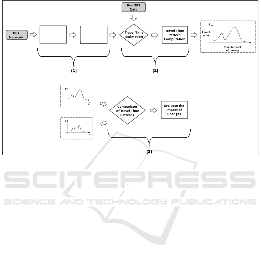
Figure 1: Stages of the approach to evaluate the impact on travel time of bus network changes.
Furthermore, to compare different versions of
travel time patterns, given two functions representing
the travel time patterns before and after any changes
in the bus network, we estimate the variation on travel
time between them by computing the area of the
region between the function values.
Lastly, we observe that some changes in the road
network may not produce structural changes in the
bus network, but produce changes in traffic patterns.
Examples are the introduction of preferential bus
lanes and the construction of new road lanes. In such
cases, Stage 1 is computed only once for both
network versions.
4 MONITORED NETWORK
In this section, we present the algorithms for selecting
the road segments whose traffic will be monitored
with the help of bus trajectories.
Specifically, Algorithm 1 computes the monitored
bus network, Algorithm 2 selects candidates for
monitored paths, and Algorithm 3 refines the
candidate monitored paths points.
4.1 Computation of the Monitored Bus
Network
We recall that, intuitively, the monitored bus network
is the set of the road segments most traversed by
buses. Algorithm 1 computes the monitored bus
network as follows.
Select the Most Traversed Road Segments. The
algorithm receives as input the bus network. Line 2
ranks the edges by the number of bus routes that
traverse them and returns the most traversed edges.
Find Connected Components. For each edge in the
set of the most traversed edges, Lines 5 and 6
compute the initial and final nodes of the edge, and
Line 9 performs a reverse breadth-first search (BFS)
over the bus network starting from the initial node of
the edge. Line 10 executes a direct BFS starting from
the final node of the edge. Both modifications of BFS
algorithm (reverse BFS and direct BFS) explore the
neighbour edges first, before moving to the next level
neighbours and they are including in the result set the
edges that are served by the same set of bus routes
that serve the most traversed edge under analysis.
When an edge served by a different set of bus routes
is encountered, the algorithms stop. Thus, the
algorithms form sub-paths composed by connected
edges that are served by the same bus routes. As a
Bus
Network
Segmentation
Monitored Bus Network B
1
Monitored Bus Network B
2
Bus
Network
Definition
An Approach to Evaluate the Impact on Travel Time of Bus Network Changes
25

Algorithm 1: Computation of the Monitored Road Network.
result of both searches, two sub-paths are obtained.
Line 11 combines both sub-paths and the edge under
analysis to compose a subgraph. As new edges are
founded by the direct and reverse BFS, they are
removed from bus network and from the list of most
traversed edges to avoid infinite loops. Lines 12 to 19
then gradually reduce the bus network and the list of
the most traversed edges until they are empty. Line
20 adds each subgraph, generated by each of the most
traversed edge, to a set of subgraphs. The same
process (Line 4 - 20) is repeated until all edges in the
most traversed set are analysed. Line 22 calls a
function to find, within the set of subgraphs, those
that have a common node and joins them in a single
connected component. Thus, a set of disjoint
subgraphs is obtained, which is the monitored road
network. Finally, Line 23 returns the monitored road
network, represented by its connected components.
4.2 Segmentation
To segment the monitored bus network, we use the
concept of control points. Then, monitored paths
composed by a sequence of connected road segments
are obtained, which are the minimal unit for
monitoring the behaviour of buses.
Algorithm 2: Computation of the candidate control points.
Algorithm 2 determines control points in the
monitored bus network as follows.
Cluster Edges by Bus Routes. The algorithm
receives as input the set of connected components that
form the monitored bus network. Line 4 applies a
clustering function to each connected component that
groups edges traversed by the same bus routes.
Find Disjoint Paths between the Same Cluster.
Segments that correspond to the same cluster may be
consecutive or not. If they are consecutive, they form
longer paths served by the same bus routes. Line 6
combines all such paths into the same group.
Determine the Initial and Final Nodes of Disjoint
Paths. Lines 8-9 compute the initial and final nodes.
For each path in the set disjPaths. Line 10 adds these
pairs of initial and final nodes to the list of candidate
control points and the monitored path between them.
Finally, Line 14 returns a list of candidate control
points.
However, not all control point candidates have the
same level of relevance in terms of traffic monitoring.
For instance, one may discard intermediate nodes
connecting two consecutive paths of the monitored
road network that belong to the same street. In such
cases, there is no significant difference in the bus
routes serving each path. For this reason, both paths
can be combined.
To address this issue and improve the quality of
the segmentation process of the monitored bus
network, Algorithm 3 refines the set of candidates for
control points, using data provided by the road
network map, as follows.
ICEIS 2017 - 19th International Conference on Enterprise Information Systems
26

Algorithm 3: Refine the list of candidates for control points.
Find Intermediate Nodes. Line 2 assigns to the
ctrlPts variable the list of candidate control points,
passed as input. Line 3 computes the intermediate
nodes between the list of candidates for control
points. Given two pairs of candidate control points,
an intermediate node is a node that is the end node of
one of the control points and the initial node on the
other.
Discard Non-relevant Intermediate Nodes. For
each node in the intermediate node list, Lines 5 and 6
extract, according to the direction and sense of the
street, its previous and subsequent nodes in the
monitored bus network. Neither the previous node,
nor the subsequent node must necessarily be
candidates for control points. It occurs just when the
path delimited by a pair of control points, where one
of the points is an intermediate node, encompasses
only one street segment.
Using data from the network map, a plausible
name of the street that connects the previous node
with the intermediate node can be obtained, as well as
the name of the street that connects the intermediate
node with the subsequent node. For this purpose, Line
7 and 8 call a crawler-function that processes
machine-readable road tags and the semantic
relations between them, to extract the name of the
street in question, to which two given coordinate
points belong.
Once the street names are found, Line 9
compares them. If the names are the same, both street
segments belong to the same street, and it means that
there is no change of street around the intermediate
node. Therefore, both paths, where the intermediate
node belongs can be joined into one to be monitored.
Line 10 removes the intermediate node from the list
of candidate control points. This process is repeated
until all nodes of the intermediate nodes list have been
analysed and the list of control points has been fully
Algorithm 4: Estimation of travel time.
refined. Line 12 returns the list of control points as
output.
5 TRAVEL TIME PATTERNS
Once the Monitored Bus Network is defined and
segmented, it is possible to mine the historical bus
GPS trajectory dataset to perform the following
operations: (1) estimation of the travel time that buses
take to traverse a given path, delimited by a pair of
control points, at a given time interval; and (2)
computation of the travel time patterns for a given
path at a given repeating time interval (for example,
every weekend). In this section, we implemented two
algorithms to execute these operations. The
algorithms consider that the period corresponds to a
day, divided into intervals (i.e. 24 fixed time intervals
of 1 hour each). Also, the second algorithm computes
only the average travel time, and not a generic time
travel statistics. However, we note that both
algorithms can be easily modified to account for more
general settings.
5.1 Estimating Travel Time
Algorithm 4 estimates the travel time that buses take
to traverse a monitored path delimited by a pair of
control points at a given time interval as follow.
Buffer Zone Definition: The algorithm receives as
input the monitored paths, and a period covered by
the period of the network. For each monitored path,
Line 3 extracts the LineString that joins the
consecutive geographical positions forming the path.
Line 4 creates a buffer zone around the LineString,
An Approach to Evaluate the Impact on Travel Time of Bus Network Changes
27

with a specific width. Note that the width value is
computed as the sum of the width of the street under
analysis and the GPS measurement error, which
typically ranges from 5 to 10 meters. As a result, the
buffer zone is a polygon, used to temporarily delimit
the raw bus GPS observations transmitted between a
pair of control points.
Filtering GPS Observations by Buffer Zone (Geo-
spatial Segmentation of Raw Trajectory Data).
Line 5 executes a geospatial-temporal query to
retrieve all GPS observations inside the defined
buffer zone for the specified period. This allows to
select GPS points that may not exactly fit road
geometries, without having to execute (expensive)
map-matching operations.
Travel Time Computation: Line 6 finds all distinct
buses (busLine, busId) that transmitted their positions
within the buffer zone. Line 7 repeats the loop to read
each found bus. Line 8 extracts only the observations
that correspond to trips that go in the direction from
first to second point of the pair of control points. Line
9 computes the trips. For those trips for which the first
or the last observation do not match the position of
the control points, a linear interpolation is used to
discover the timestamps when the bus passed through
the control points. Line 10-13 computes and saves the
travel time for each trip.
It is worth mentioning that Algorithm 4 computes
the travel time of trips made in the period defined by
the input parameter day , whose value may be set to
be one day or multiple days belonging to the period
of each road network stored in the dataset. To make
the computation for many days, one only has to pass
a set of days as value of the input parameter.
5.2 Computing Travel Time Patterns
Algorithm 5 computes the travel time pattern of each
path, at a given time interval. Again, for simplicity, it
considers that the period corresponds to a day,
divided into 24 fixed time intervals of 1 hour each,
but the code can be easily generalized.
The algorithm receives as input a specific day, the
paths of the monitored bus network and the intervals
dividing the day. Line 2 uses a loop to analyse each
of these paths. For each path, Line 3 retrieves the
travel time table that corresponds to the bus trips
made in the specified day. Line 5 is a second loop that
steps through each interval of the day. Line 6 recovers
trips whose time of entry into the path belongs to the
time interval being analysed. Line 7 counts the
number of these trips. The travel time pattern for this
particular interval is computed in Line 8 as the mean
Algorithm 5: Computation of the travel time pattern for all
paths of the Monitored Network during a given day.
travel time for the same path at the referred time
interval. Line 9 saves the travel time pattern for future
analysis. This process is repeated until all intervals of
the day have been examined.
Since Algorithm 5 computes the travel time
patterns of all segments of the monitored bus
network, but only for one day, it must be run for all
days belonging to the period of the road network. As
the volume of data to be processed is very large, to
reduce the execution time, a distributed algorithm has
been designed and implemented. It will not be
explained in this paper due to space limitations.
6 EXPERIMENTS
The experiments evaluated how bus travel time
patterns in the City of Rio de Janeiro were affected by
traffic changes implemented mostly for the Rio 2016
Olympic Games. To support the evaluation, a large
data set containing the GPS positions (more than 3
billion samples) of all buses that operated in the City
of Rio de Janeiro from June 12
th
, 2014 until
November 30
th
, 2016 was used. Each sample contains
a timestamp, the bus identifier, the line number, the
position (as latitude and longitude) and the speed.
The traffic changes we evaluated were: the
construction of the New Joá Elevated Road; the
introduction of exclusive bus lanes for bus rapid
service (BRS) on the Voluntários da Pátria and São
Clemente Streets; and the construction of the bus
rapid transit (BRT) corridor of the Americas Avenue.
The New Joá Elevated Road has 5 km of
extension and 2 lanes, whereas the Old Joá Elevated
Road – still in operation – has 4 lanes. They both
connect the south zone of Rio and Barra da Tijuca (a
neighbourhood in the west of Rio where the Olympic
ICEIS 2017 - 19th International Conference on Enterprise Information Systems
28

Games took place). We then have two scenarios,
which we call old and new, defined as follows:
Old scenario: just the Old Joá Elevated Road,
with 2 traffic lanes in each direction, except
during the morning traffic peak hours, when 3
lanes were used for traffic flowing from Barra da
Tijuca to the south zone;
New scenario: the Old and New Joá Elevated
Roads, which in combination offer 3 traffic lanes
in each direction, all day long; in each direction,
one of the lanes is reserved for cars. There is no
use of a reverse lane in the morning.
The bus routes connecting the south zone and
Barra da Tijuca greatly benefited from this new traffic
scenario. Our experiments focused on the bus traffic
from Barra da Tijuca to the south zone, with emphasis
on the morning peak hours.
The construction of the New Joá Elevated Road
started at the end of June 2014, and the new road was
inaugurated on May 28
th
, 2016. In our evaluation, we
considered two periods: from June 12
th
, 2014 to May
27
th
, 2015; and from May 28
th
, 2016 to November
30
th
, 2016. All trajectories in the period from May
27
th
, 2015 to May 28
th
, 2016 – the peak of the
construction of the new road – were eliminated from
the sample to avoid introducing noise in the
computation of travel time.
To execute Stage 2 of the approach (see Figure 1),
we selected a path of the monitored network that goes
from Ministro Ivan Lins Avenue to the Gávea Road
(in the direction from Barra de Tijuca to the south
zone). This path was heavily affected by the
construction of the new elevated road.
For the old scenario, we analysed a total of 24,846
trajectories, generated by 1,011 buses, serving 70
daily routes, that cover the path under study.
Corresponding to the new scenario, we analysed a
total of 8,310 trajectories, generated by 115 buses
serving 66 daily routes.
Since the travel times in weekdays differ
dramatically from weekends, within the same
scenario, we analysed these periods separately.
Figure 2a shows the travel time patterns for the
weekdays belonging to the old scenario (v1) versus
the new scenario (v2), while Figure 2b depicts the
travel time patterns for the weekends.
At Stage 3 of the approach, we computed the area
between the two curves during the morning peak
hours (from 6 to 10 o'clock). The result was 15.00.
This means an average reduction of the travel time in
the morning peak hours by approximately 4 minutes.
As the graphs in Figure 2a corroborate, there are
significant variations in travel time from one pattern
to the other, specifically at the peak hours in the
morning (from 6 to 10 o'clock), when the flow of
vehicles in the direction Barra de Tijuca - south zone
is larger than during the rest of the day. The results of
the experiments then demonstrate that the
commissioning of the New Joá Elevated Road
produced significant a reduction of bus travel time
from Barra da Tijuca to the south zone.
The experiments related to the introduction of the
preferential bus lane on the Voluntários da Pátria and
São Clemente Streets on August 2
th
, 2014 indicated
that these changes did not produce significant benefits
in terms of the reduction of bus travel time. By
contrast, the BRT corridor on the Americas Avenue,
inaugurated on August 23
th
, 2016 reduced bus travel
time by 45%. The results of these experiments were
omitted due to space limitations.
7 RELATED WORK
We review work which is closely related to our study,
divided in: (i) segmentation of raw trajectories; (ii)
estimation of traffic patterns from GPS data; and (iii)
traffic impact of road network changes.
Segmentation of Raw Trajectories. There are
different criteria to segment raw trajectories. They
range from the transportation means used (Biljecki et
al. 2013), potential-transition locations (e.g. bus
stops) (Liao et al. 2006), geo-spatiotemporal
information (Buchin et al. 2011), detection of similar
sub-trajectories (Sankararaman et al. 2013) and
movement analysis (Alewijnse et al. 2014). In this
paper, we specifically discuss how to segment row
trajectories based on the passing of buses by control
points.
Extraction of Traffic Patterns from GPS Data.
Multiple traffic patterns can be estimated using
historical GPS trajectory data, such as: traffic flow,
traffic demand and travel time. The extraction of
these traffic patterns pursues two main objectives: to
explain common traffic conditions and to predict
future traffic conditions. Work focused on the first
objective addresses traffic monitoring [Blind1],
detection of traffic anomalies (Kuang et al. 2015),
traffic performance analysis (Shi et al. 2008). Work
focused on the second objective includes traffic state
prediction (Zhang et al. 2013), urban traffic
congestion forecasting (Hou et al. 2012; Kong et al.
2016), prediction of traffic anomaly duration (Li
2015) and estimating time of arrival (Coquita et al.
2015; Kormáksson et al. 2014; Jithendra. H. K 2015).
This paper is targeted at the first objective,
specifically to model past and current traffic
behaviour based on travel time patterns.
An Approach to Evaluate the Impact on Travel Time of Bus Network Changes
29

Traffic Impact of Bus Network Changes. There
have been a variety of bus priority strategies adopted
to reduce bus travel time delays, increase passenger
comfort and thereby improve public transportation
service quality. Studies assessing the implementation
impacts of some of these strategies analyze: traffic
signal priority for buses (Daniel et al. 2004),
exclusive bus lanes (Chen et al. 2016), bus lane
combinations (Truong et al. 2015; Fowkes et al.
2014), bus rapid transit (BRT) implementation
(Carrigan et al. 2013), bus operation in platoon
(Shrestha et al. 2009). More comprehensive studies
(Bhattacharyya et al. 2016) analyse the effects of
multiple bus priority treatments simultaneously. This
paper focuses on the evaluation of travel time impacts
of various bus network changes implemented in the
City of Rio de Janeiro mostly for the Rio 2016
Olympic Games.
8 CONCLUSIONS
In this paper, we proposed an approach to evaluate the
impact of bus network changes on bus travel time.
The approach relies on data obtained from buses
equipped with GPS devices, which act as mobile
traffic sensors. This type of study allows analyzing
the evolution of the city with respect to urban
mobility in a systematic way, similarly to the analysis
of population growth and occupation of land made
with satellite images. It also provides urban planners
unprecedented opportunities for better understanding
urban transportation system and for better exploiting
the knowledge thereof.
Using the proposed approach, we investigated the
effect on bus travel time of traffic changes
implemented in the City of Rio de Janeiro mostly for
the Rio 2016 Olympic Games.
Directions for future research include the
estimation of the impact of road network changes on
traffic flow. In this context, statistical quality control
to evaluate current conditions with respect to normal
condition based on historical data will be applied. We
are also implementing a traffic observatory that will
help city planner analyze bus network changes and
that will include a real-time component to help alert
city authorities about anomalous traffic conditions.
REFERENCES
Alewijnse, S. et al., 2014. A framework for trajectory
segmentation by stable criteria. Proc. 22nd ACM
SIGSPATIAL Int'l. Conf. on Advances in Geographic
Information Systems.
Bhattacharyya, K., Maitra, B. & Boltze, M., 2016. Qualitative
analysis for selection of bus priority techniques and
operational strategies in the context of emerging countries.
World Conference on Transport Research.
Biljecki, F., Ledoux, H. & Van Oosterom, P., 2013.
Transportation mode-based segmentation and
classification of movement trajectories. Int'l. J. of
Geographical Information Science.
Buchin, M. et al., 2011. Segmenting trajectories: A framework
and algorithms using spatiotemporal criteria. Journal of
Spatial Information Science.
Carrigan, A. et al., 2013. Social, environmental and economic
impacts of BRT systems. Bus Rapid Transit Case Studies
from Around the World.
Chen, Y., Chen, G. & Wu, K., 2016. Evaluation of
Performance of Bus Lanes on Urban Expressway Using
Paramics Micro-simulation Model. Procedia Engineering.
Coquita, K. et al., 2015. Prediction System of Bus Arrival Time
Based on Historical Data Using Regression Models. Proc.
XI Brazilian Symp. on Information Systems (SBSI 2015).
Daniel, J. et al., 2004. Assess impacts and benefits of traffic
signal priority for buses.
Feitelson, E. & Rotem-Mindali, O., 2015. 19 Spatial
implications of public transport investments in
metropolitan areas: some empirical evidence regarding
light rail and bus rapid transit. International Handbook on
Transport and Development.
Fowkes, N.D. et al., 2014. The effect of allowing minibus taxis
to use bus lanes on rapid transport routes.
Hou, L. et al., 2012. Estimation of incident-induced congestion
on signalized arteries using traffic sensor data. Tsinghua
Science and Technology.
Jepson, D. & Ferreira, L., 1999. Assessing travel time impacts
of measures to enhance bus operations. Part I: Past
Evidence and Study Methodology. Road and Transport
Research: a journal of Australian and New Zealand
research and practice.
Jepson, D. & Ferreira, L., 2000. Assessing travel time impacts
of measures to enhance bus operations. Part II: Assessment
criteria and main findings. Road and Transport Research:
a journal of Australian and New Zealand research and
practice.
Jithendra. H. K, N.R.K.D., 2015. Predicting Bus Arrival Time
based on Traffic Modelling and Real-time Delay. Int'l. J.
of Engineering Research & Technolog.
Kong, X. et al., 2016. Urban traffic congestion estimation and
prediction based on floating car trajectory data. Future
Generation Computer Systems.
Kormáksson, M. et al., 2014. Bus travel time predictions using
additive models. Proc. 2014 IEEE Int'l. Conf. on Data
Mining.
Kuang, W., An, S. & Jiang, H., 2015. Detecting traffic
anomalies in urban areas using taxi GPS data.
Mathematical Problems in Engineering.
Li, R., 2015. Traffic incident duration analysis and prediction
models based on the survival analysis approach. IET
Intelligent Transport Systems.
Liao, L. et al., 2006. Building personal maps from GPS data.
Annals of the New York Academy of Sciences.
ICEIS 2017 - 19th International Conference on Enterprise Information Systems
30

Lindau, L.A. et al., 2014. BRT and bus priority corridors:
Scenario in the American continent. In Transportation
Research Board 93rd Annual Meeting.
Sankararaman, S. et al., 2013. Model-driven matching and
segmentation of trajectories. In Proceedings of the 21st
ACM SIGSPATIAL International Conference on Advances
in Geographic Information Systems.
Shi, W., Kong, Q.-J. & Liu, Y., 2008. A GPS/GIS integrated
system for urban traffic flow analysis. Proc. 2008 11th Int'l.
IEEE Conf. on Intelligent Transportation Systems.
Shrestha, P.K., Nakamura, F. & Okamura, T., 2009. Study on
operation and performance of bus priority policies
considering intended platooning of bus arrivals. Civil
Engineering Studies Research Papers.
Truong, L.T., Sarvi, M. & Currie, G., 2015. Exploring
Multiplier Effects Generated by Bus Lane Combinations.
Transportation Research Record: J. of the Transportation
Research Board.
Alewijnse, S. et al., 2014. A framework for trajectory
segmentation by stable criteria. Proc. 22nd ACM
SIGSPATIAL Int'l. Conf. on Advances in Geographic
Information Systems.
Arasan, V.T. & Vedagiri, P., 2010. Study of the impact of
exclusive bus lane under highly heterogeneous traffic
condition. Public transport.
Bhattacharyya, K., Maitra, B. & Boltze, M., 2016. Qualitative
analysis for selection of bus priority techniques and
operational strategies in the context of emerging countries.
World Conference on Transport Research.
Biljecki, F., Ledoux, H. & Van Oosterom, P., 2013.
Transportation mode-based segmentation and
classification of movement trajectories. Int'l. J. of
Geographical Information Science.
Buchin, M. et al., 2011. Segmenting trajectories: A framework
and algorithms using spatiotemporal criteria. Journal of
Spatial Information Science.
Carrigan, A. et al., 2013. Social, environmental and economic
impacts of BRT systems. Bus Rapid Transit Case Studies
from Around the World.
Chen, Y., Chen, G. & Wu, K., 2016. Evaluation of
Performance of Bus Lanes on Urban Expressway Using
Paramics Micro-simulation Model. Procedia Engineering.
Coquita, K. et al., 2015. Prediction System of Bus Arrival Time
Based on Historical Data Using Regression Models. Proc.
XI Brazilian Symp. on Information Systems (SBSI 2015).
Currie, G., 2006. Bus rapid transit in Australasia: Performance,
lessons learned and futures. J. of Public Transportation.
Daniel, J. et al., 2004. Assess impacts and benefits of traffic
signal priority for buses.
Deng, T. & Nelson, J.D., 2013. Bus Rapid Transit
implementation in Beijing: An evaluation of performance
and impacts. Research in Transportation Economics.
Feitelson, E. & Rotem-Mindali, O., 2015. 19 Spatial
implications of public transport investments in
metropolitan areas: some empirical evidence regarding
light rail and bus rapid transit. International Handbook on
Transport and Development.
Fowkes, N.D. et al., 2014. The effect of allowing minibus taxis
to use bus lanes on rapid transport routes.
Hou, L. et al., 2012. Estimation of incident-induced congestion
on signalized arteries using traffic sensor data. Tsinghua
Science and Technology.
Jithendra. H. K, N.R.K.D., 2015. Predicting Bus Arrival Time
based on Traffic Modelling and Real-time Delay. Int'l. J.
of Engineering Research & Technolog.
Kong, X. et al., 2016. Urban traffic congestion estimation and
prediction based on floating car trajectory data. Future
Generation Computer Systems.
Kormáksson, M. et al., 2014. Bus travel time predictions using
additive models. Proc. 2014 IEEE Int'l. Conf. on Data
Mining.
Kuang, W., An, S. & Jiang, H., 2015. Detecting traffic
anomalies in urban areas using taxi GPS data.
Mathematical Problems in Engineering.
Li, R., 2015. Traffic incident duration analysis and prediction
models based on the survival analysis approach. IET
Intelligent Transport Systems.
Liao, L. et al., 2006. Building personal maps from GPS data.
Annals of the New York Academy of Sciences.
Lindau, L.A. et al., 2014. BRT and bus priority corridors:
Scenario in the American continent. In Transportation
Research Board 93rd Annual Meeting.
Sankararaman, S. et al., 2013. Model-driven matching and
segmentation of trajectories. In Proceedings of the 21st
ACM SIGSPATIAL International Conference on Advances
in Geographic Information Systems.
Shalaby, A.S. & Soberman, R.M., 1994. Effect of with-flow
bus lanes on bus travel times. Transp. research record.
Shi, W., Kong, Q.-J. & Liu, Y., 2008. A GPS/GIS integrated
system for urban traffic flow analysis. Proc. 2008 11th Int'l.
IEEE Conf. on Intelligent Transportation Systems.
Shrestha, P.K., Nakamura, F. & Okamura, T., 2009. Study on
operation and performance of bus priority policies
considering intended platooning of bus arrivals. Civil
Engineering Studies Research Papers.
Truong, L.T., Sarvi, M. & Currie, G., 2015. Exploring
Multiplier Effects Generated by Bus Lane Combinations.
Transportation Research Record: J. of the Transportation
Research Board.
Zhang, J.-D., Xu, J. & Liao, S.S., 2013. Aggregating and
sampling methods for processing GPS data streams for
traffic state estimation. IEEE Transactions on Intelligent
Transportation Systems.
An Approach to Evaluate the Impact on Travel Time of Bus Network Changes
31
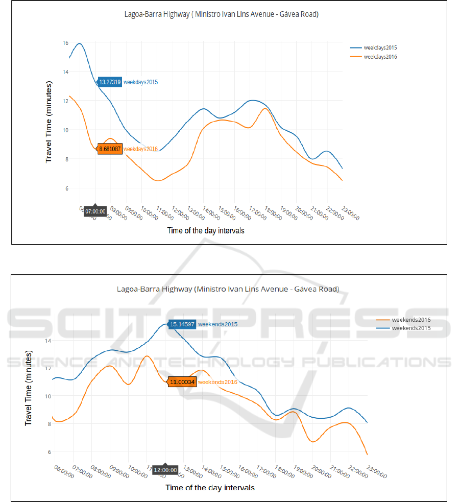
Figure 2a: Travel Time Patterns for weekdays of v1 vs v2 Lagoa - Barra Highway.
Figure 2b: Travel Time Patterns for weekends v1 vs v2 Lagoa - Barra Highway.
ICEIS 2017 - 19th International Conference on Enterprise Information Systems
32
