
Data Warehouse MFRJ Query Execution Model for MapReduce
Aleksey Burdakov, Uriy Grigorev, Victoria Proletarskaya and Artem Ustimov
Bauman Moscow State Technical University, 2
nd
Baumanska 5/1, Moscow, Russia
Keywords: MapReduce, Data Warehouse, MFRJ Access Method, Analytical Model, Adequacy.
Abstract: The growing number of MapReduce applications makes the Data Warehouse access time estimating an
important task. The problem is that processing of large data requires significant time that may exceed the
required thresholds. Fixing these problems discovered at the system operations stage is very costly. That is
why it is beneficial to estimate the data processing time for peak loads at the design stage, i.e. before the
MapReduce tasks implementation. This allows making timely design decisions. In this case mathematical
models serve as an unreplaceable analytical instrument. This paper provides an overview of the n-dimensional
MapReduce-based Data Warehouse Multi-Fragment-Replication Join (MFRJ) access method. It analyzes
MapReduce workflow, and develops an analytical model that estimates Data Warehouse query execution
average time. The modeling results allow a system designer to provide recommendations on the technical
parameters of the query execution environment, Data Warehouse and the query itself. This is important in
cases where there are restrictions imposed on the query execution time. The experiment preparation and
execution in a cloud environment for model adequacy analysis are evaluated and described.
1 INTRODUCTION
Data Warehouses are commonly used for Big Data
processing (Kaur, 2016) and are especially popular in
Business Intelligence applications (Duda, 2012).
They support a multi-dimensional model (Inmon,
2005; Golfarelli and Rizzi, 2009). A Data Warehouse
with dimensions has the form of a multi-dimensional
cube. Every point in this cube corresponds to one or
multiple values (facts). Sparse data cubes are allowed.
Data Warehouse implementation principles
varied over time. There were three approaches at the
beginning: MOLAP, ROLAP, HOLAP (Inmon,
2005; Golfarelli and Rizzi, 2009; Duda, 2012).
MOLAP (Multidimensional OnLine Analytical
Processing) data is stored in the form of special
ordered multidimensional arrays (hypercubes and
polycubes). ROLAP (Relational OLAP) uses a
relational database to store dimension and fact tables.
HOLAP (Hybrid OLAP) combines the two above
mentioned approaches. The following products
implement these approaches: Oracle Hyperion
Essbase (MOLAP), MS SQLServer 2000 Analysis
Services (MOLAP, ROLAP or HOLAP), et.al.
However, with the growth of the processed data
volumes the Data Warehouse implementation cost
has also radically increased (Hejmalíček, 2015).
Regularly the platform for large Data Warehouse
implementation is RDBMS (Relational DataBase
Management System). In order to significantly
increase the volume of processed data an additional
powerful server(s) has to be added (which is costly)
as well as purchasing an additional license for
installation of a new RDBMS entity. Moreover,
additional costly software has to be installed to
support distributed environment and optimize Data
Warehouse processes. One of the most expensive
Data Warehouse parts is its external memory. The
disks are organized into a RAID to ensure fault
tolerance leading to expensive planning and support.
The Data Warehouse strategy has changed with
the emergence of NoSQL databases (Duda, 2012).
This can be attributed to the fact that NoSQL are open
source systems with great scalability (up to a few
thousand nodes) and reliability (due to multiple
replication of database records) as well as low node
cost (Redmond and Wilson, 2012; Sadalage and
Fowler, 2012). Already existing platforms were used
initially. They read actual data with ETL from a
NoSQL database into a MOLAP cube and process it
there, e.g. Jaspersoft and Pentaho (Duda, 2012).
However, here the volume of processed data was
limited by the single MOLAP server.
206
Burdakov, A., Grigorev, U., Proletarskaya, V. and Ustimov, A.
Data Warehouse MFRJ Query Execution Model for MapReduce.
DOI: 10.5220/0006238502060215
In Proceedings of the 2nd International Conference on Internet of Things, Big Data and Security (IoTBDS 2017), pages 206-215
ISBN: 978-989-758-245-5
Copyright © 2017 by SCITEPRESS – Science and Technology Publications, Lda. All rights reserved

MapReduce (MR) (Jeffrey and Sanjay, 2004;
Duda, 2012; Hejmalíček, 2015) became the next step
of Data Warehouse evolution. There are many
technologies based on MR that allow implementation
of a Data Warehouse (Li, et.al, 2014). Hive is an
example of major Facebook platform components. It
is intended for implementation of a Data Warehouse
in Hadoop (Huai, et al., 2014). Here a SQL query is
translated into a series of MR tasks. Some
experiments show that Hive is significantly slower
than other methods (Duda, 2012; Zhou and Wang,
2013). In order to solve the low performance problem
of a Data Warehouse in MR systems some methods
were developed that allow access to Data Warehouse
directly in MR (i.e. without additional components).
Four such methods (MFRJ, MRIJ, MRIJ on RCFile,
MRIJ with big dimension tables) are described in
(Zhou and Wang, 2013). They are based on the
dimension table caching in the RAM of each node.
Along with the MR Hadoop a MapReduce-like
system Spark and others are used; however, their
discussion is outside of this paper’s scope.
This paper discusses Multi-Fragment-Replication
Join (MFRJ) method (Zhou and Wang, 2013), which
unlike other methods allows access to n-dimensional
Data Warehouse for only one MR task and avoids
extra transfers of the fact table external keys (section
3). It is also simple in implementation. Effectiveness
of this method in comparison with other methods is
shown in (Zhou and Wang, 2013).
The motivation of this work is the need for Data
Warehouse access time forecasts, due to the intense
growth in number of MR applications. Examples of
such applications are provided below:
o Internet-application log processing for large
internet shops and social networks (Duda,
2012) for service demand analysis.
o Large data volume processing for data
collected by credit organizations for market
behavior forecasts.
o Statistics calculation for large weather
forecast processing.
The problem is that large volume data processing
is time-consuming which may become unacceptable.
Discovery of this problem at the operational stage
leads to costly resolution. First of all, there are many
processing tasks. Secondly, if the tasks are complex
then tuning does not help. In this case algorithms
have to be changed and Map and Reduce functions
recoded. This means redoing the already done work
wasting time and resources. Thus the processing time
estimation for peak load during the design stage, i.e.
before MR tasks implementation, is beneficial.
The importance of modeling can be demonstrated
on the following example. Two RDBMSes (column
and row-based) and MR Hadoop were compared in
an experiment in (Pavlo, et.al, 2009). The conclusion
was that Hadoop loses in the test tasks.
Detailed analysis in (Burdakov, et.al, 2014)
showed that experiments with RDBMS were
executed with the node number below 100, with low
data selectivity in queries, with the lack of sorting,
and record exchange of fragmented tables between
the nodes. Modeling was performed with calibrated
models and different input parameters (Burdakov,
et.al, 2014). The results showed that Hadoop over-
performing RDBMS with high selectivity and sorting
starting from 300 nodes (6 TB of stored data).
Obviously, implementation of a test stand and live
experiments on a large number of nodes is much more
expensive than development of an adequate
mathematical model and its application.
This paper discusses an MFRJ access method to a
Data Warehouse (section 3), analyzes MR workflow
(section 4), develops an analytical model for Data
Warehouse query execution time evaluation (section
5), and calibrates the model and evaluates its
adequacy based on experiments (section 6).
2 RELATED WORK
The developed analytical model for query execution
time evaluation is a cost model (Simhadri, 2013).
Below we provide an overview of the existing
models and point out their disadvantages.
Burdakov, et.al (2014) and Palla (2009) model
only two tables join in MR. Palla (2009) evaluates
input/output cost, but disregards the processing part.
However, as the measurements indicate (e.g. see
Section 6), the process load cannot be disregarded.
The processing time is considered in (Burdakov, et.al,
2014), however the Shuffle algorithm is simplified.
Afrati and Ullman (2010) propose the following
access method to n-dimensional Data Warehouses.
The Map phase in each node reads dimension and fact
table records (n+1 tables). The Map function
calculates hash-values h(b
i
) for b
i
attributes that
participate in a join. Each Reduce task is associated
with n values {h(b
i
)}. Each record is sent to multiple
Reduce tasks according to the calculated hash-values.
The Reduce task joins received records. Transferred
records number minimization task is solved based on
a constant number of Reduce tasks. This method has
the following disadvantages:
Data Warehouse MFRJ Query Execution Model for MapReduce
207

1) It assumes record transfer of the joined tables
between the nodes which may consume
significant time.
2) In certain cases the optimization task does not
have an acceptable solution.
An example for query execution time in a Hadoop
Data Warehouse provided in (Afrati and Ullman,
2010) has 2052 sec duration (two dimensions, one
fact table, four nodes, 100 Reduce tasks and
approximately one million records in each table).
An n-dimensional Data Warehouse query
execution optimization method is provided in (Wu,
et.al, 2011). An optimal plan is defined for a received
query. Each option’s cost is evaluated taking into
account record duplication as in (Afrati and Ullman,
2010). This method has the following disadvantages:
1) Histograms are built for table columns before
the optimization;
2) Record duplication throughout nodes is
required;
3) The weights for the cost model have to be
defined manually;
4) The fact that the processes in resources at the
Shuffle phase are executed in parallel;
5) Disregards the split number, Java Virtual
Machine (JVM) containers number per node,
and that the Reduce-side sort merge can have
a few execution rounds.
Zhou & Wang (2013) provide simplified estima-
tion formulas for RAM and data volumes read from a
disk and transferred through a network. However,
these formulas do not account for MapReduce
process functioning specifics (see section 4).
Afrati, et.al, (2012) evaluate the following two
MR characteristics for different tasks: average
number of records generated by Map tasks for each
input (replication rate); the list upper border for
values linked with a key (reducer size). The Reduce
task load is evaluated based on these characteristics.
The theoretical works (Karloff, et.al, 2010;
Koutris and Suciu, 2011) build abstract MR models.
The estimates are given at the asymptotic record form
level (O(n), Ω (n), etc.), that cannot be used for
concrete calculations. The work (Tao, et.al, 2013)
defines conditions when MR algorithms (sorting,
etc.) satisfy the following minimal algorithm
conditions: Minimum Footprint, Bounded Net-traffic,
Constant Round, and Optimal Computation.
The model developed in this paper has the
following advantages:
1) It models MFRJ algorithm behavior where it
is not required to duplicate Data Warehouse
table records.
2) It is not required to manually assign weights
for cost estimate.
3) The model calculates average volume-
temporal characteristics of query execution
in n-dimensional Data Warehouses
(considering disk, processor and network).
4) It is detailed, accounts for specifics of Map,
Shuffle and Reduce phases, and can be tuned
for a large number of parameters influencing
the temporal characteristics (section 5).
5) It has a parameters calibration procedure.
3 MFRJ DATA WAREHOUSE
ACCESS METHOD IN
MAPREDUCE ENVIRONMENT
The query execution algorithm in n-dimensional Data
Warehouses with the use of the MFRJ method (Zhou
and Wang, 2013) is discussed below.
SELECT D
1
.d
11
, D
2
.d
21
, …, D
n
.d
n1
,
F.m
1
, … F.m
k
FROM D
1
JOIN F ON (D
1
.d
10
= F.fk
1
)
JOIN D
2
ON (D
2
.d
20
= F.fk
2
)…
JOIN D
n
ON (D
n
.d
n0
= F.fk
n
) (1)
WHERE CD1 AND CF1,
where D
1
, …., D
n
are dimension tables, F is a fact
table, CD1 and CF1 are some additional conditions,
applied to dimensions and facts.
Figure 1: Fact table decomposition into 1+k tables (Zhou
and Wang, 2013).
The dimension tables are duplicated on all
Hadoop system nodes. They are stored in rows. The
fact table is divided into 1+k tables (see Figure 1): the
1st row includes columns of external dimension keys
(fk
i
), every fact column (m
i
) comprises a separate
table (tables 2,…,к+1). All table blocks 1…k+1 are
IoTBDS 2017 - 2nd International Conference on Internet of Things, Big Data and Security
208

arbitrarily and automatically spread throughout the
nodes by Hadoop (Hadoop attempts to make it even).
The data access is executed in the following
manner for the query type (1):
Map (in each node):
1) Records are read from dimension tables that
participate in a query. The CD1 condition is checked
for each record. Hash-indices are built in RAM for
records satisfying the condition.
2) Dimension external keys of fact tables
(Table 1) that are stored in (fk
i
) nodes are read; each
row (position) and external key is checked for
existence of the key in the corresponding hash-index;
upon successful comparison the following record is
put into the output stream:
<position1,(vd
1
,…,vd
n
)> (2)
where «position1» is a row number in external key
table (the enumeration is continuous for table 1 rows);
(vd
1
,…,vd
n
) is a list of attribute values of dimension
tables that are given in (1) following SELECT (they
are selected from dimensions hash-indices).
3) The i-th fact column values are read (table i+1)
that are stored in a node; for each fact value the CF1
query condition is checked and its value is put into the
output stream:
<position 2i, vm
i
>, (3)
where «position 2i» is the row number in i+1 table
(continuous enumeration for all i+1 table rows), vm
i
is the i-th fact value.
The «position 1» and «position 2i» key values
correspond to one fact table, however by conditions
the 1…k+1 table blocks are arbitrarily spread by
nodes.
4) The item 3 is further repeated for other fact
columns which blocks are stored in the node
(i=1,…,k).
Reduce:
If the element number of the value area of the
record received by Reduce function (after grouping
by position) equals to n+k (n is the number of
dimensions, k is the number of facts) and it satisfies
the query condition (relationships between columns
are checked), then the record is put into the output
stream as the resulting table row:
<position, (vd
1
,…,vd
n
,vm
1
,…,vm
k
)> (4)
The MFRJ method was implemented in Hadoop
environment.
4 MAPREDUCE SYSTEM
FUNCTIONING PROCESS
Map Phase (see Figure 2). L entities of Map function
are simultaneously run on each of N
M
nodes (label 2;
the labels on the Figure 2 are underlined). The Map
entities are executed simultaneously and read MR
records (objects) from the MR file system in
<key,value> pairs (label 1).
Each Map entity processes records of one
input file. The size of the processes partition does not
exceed the size of one split (by default its size is equal
to the block size V
S
=V
B
= 128 MB). Upon completion
of the Map entity another entity is started that
processes the next split file, and so on (if Map number
per node is higher than L). Overall
SF
V/V
Map
entities will be executed on one node for each input
file, where V
F
is the input file volume on that node.
The received records are converted into new
<key1,value1> records and are stored into a RAM
buffer (label 3). A Q
B
-sized RAM buffer is allocated
to each Map entity. Once the buffer is saturated, a
new thread is started in the background. It splits the
buffer into fragments and sorts each fragment by key
(in-memory sort). The number of fragments in the
buffer equals s number of partitions (Reduce task
entities) set in a Job. A record belongs to i-th buffer
fragment (i.e. to i-th partition) if h(attribute)=i where
h is a hash-function. After that each sorted buffer
fragment is output to the disk as part of a file (spill to
disk) (label 4). So, the total number of sorted
fragments that will be stored on a disk during the
execution of one Map node entity will be equal to r
multiplied by s, where r is the number of stored files
determined by the following formula:
r= Q/( Q
B
·P
T
·P
M
/16)=Q/Q
M
, (5)
where Q is the total number of output records
generated by one Map function entity (i.e. per one
split), Q
B
is the RAM buffer size (100 MB by default),
P
T
is the buffer fill threshold (0.8), P
M
is a part of the
buffer allocated for metadata (0.05), 16 is the
metadata record size in bytes (Palla, 2009).
Note: Fragments (j-1)s+1,…, js are parts of j-th
file, j=1…r (see Figure 2, label 4). So r physical files
are stored on a disk, each of which has s logical files
(fragments).
Data Warehouse MFRJ Query Execution Model for MapReduce
209
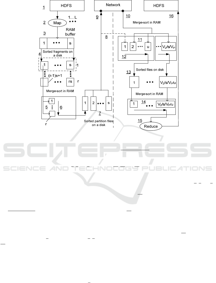
Figure 2: MapReduce operation execution sequence.
Once the Map function has processed all input records
of its split, a special procedure is started on the node.
It reads i-th partition fragments and outputs them into
one sorted file (merge on disk, labels 5, 6 and 7). This
file is sorted by the key «key1». The procedure
described above is executed consequently for all
partitions (i=1,…,s) of Map entity.
The activities described above are executed in
parallel for all Map entities simultaneously executed
on the node. The sorting is necessary for group
operation execution at the Reduce phase.
Shuffle Phase. The master nodes are informed on
Map entity execution completion. Simultaneously
with Map R entities of Reduce task are started on each
of N
R
nodes. Each j-th Reduce task queries the master
node, determines the completed Maps and reads j-th
partition files (see label 7) into its area (labels 8, 9 and
10). So, the different nodes’ files with one partition
number j will be transferred into a node where the j-
th Reduce task is executed (j=1,…,s). If the file size
is below 0.7·0.25·V
HR
, then it is stored in a Reduce
and Map JVM heap. By default its size is 200 MB. If
the size of a filled heap exceeds the V
P
=0.7·0.66·V
HR
threshold, then the files stored in the heap are merged
into one file stored on a disk (similar to label 6).
The above description tells us that Map and
Shuffle intersect. Li, et.al (2011) and analysis of logs
generated by Hadoop query execution confirm that.
Reduce Phase. If the number of saved files
exceeds the 2(u-1) threshold, then «u» files are
merged into one file and it is stored on a disk (labels
11, 12 and 13). By default u=100, V
2
is the input data
volume of all Reduce tasks. This case is possible if a
significant data volume is processed by a cluster with
a small number of nodes (similar to labels 5, 6 and 7).
The stored files are read and sorted/merged in
RAM (label 14), so that one sorted flow of records is
formed. The system groups the records of the stream
by the values of the key that was used for sorting
(label 15). Record groups are sent to the Reduce
function input without its intermediate disk storage.
The Reduce function then processes each group
and puts the result into the output stream. This data is
stored in the MR file system (label 16).
5 DATA WAREHOUSE
AVERAGE ACCESS TIME
ESTIMATE FOR MFRJ
METHOD
The Figure 3 depicts the analytical model structure for
Data Warehouse query execution time calculation
(MapReduce task) for the MFRJ method.
IoTBDS 2017 - 2nd International Conference on Internet of Things, Big Data and Security
210
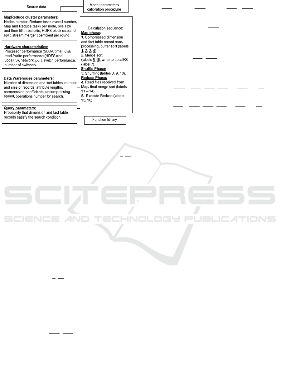
Figure 3: Analytical model structure.
The model is developed based on the MR
workflow description (Section 4). The labels (1-16)
on Figure 3 correspond to the labels on Figure 2. The
model calculates time-volume characteristics for each
phase (Map, Shuffle, Reduce) and the whole task.
The models shall be calibrated based on task
execution time measurements since it is impossible to
directly measure some input parameters of the model.
For example the model takes into account the
processor portion of the MapReduce task execution
time. One short logical operation execution time of an
algorithm (SLOA) is set as a parameter (Burdakov,
et.al, 2014), which is challenging to measure. Model
calibration allows evaluation of that parameter.
The model is rather complex as it accounts for
MapReduce parallel processing specifics. Due to the
space restrictions we provide only one formula
fragment. Below there is a fragment that calculates
Shuffle time (labels 8-10 on Figure 2). The resource
processes at the Shuffle phase are executed in
parallel, so the time is defined by the slowest re-
source, and hence the max function is used. Formula
(6 a-g) define the resource temporal characteristics:
max)G,(VT
22
N
SH
=
{ (6)
dRM
2
μ
1
N
V
⋅
, (a)
PW
M
μ
1
V ⋅
, (b)
N1R
M
MR
μ
1
)
N
1
(VK
N
N
1)(K
N
N
⋅⋅⋅−
, (c)
N2R
M
MR
μ
1
)
N
1
(VN
N
N
K)(N
N
N
⋅⋅⋅−
, (d)
PR
R
μ
1
V ⋅
, (e)
)/VV(/s)log(Gk6.5τ
2FP22
⋅⋅⋅
, (f)
dWR
2
μ
1
N
V
⋅
}, (g)
where
)
N
1
1(
N
V
)
N
1
N
V
(
N
N
N
V
V
M
2
RM
2R
M
2
M
−=⋅−=
, (7)
)
N
1
1(
N
V
)
N
1
N
V
(
N
N
N
V
V
R
2
RM
2M
R
2
R
−=⋅−=
, (8)
)/s/V/(VVV
S122F
=
. (9)
The equations (6)-(9) use the following notations:
N is the total number of nodes; N
M
is the number of
nodes that execute the Map tasks (N
M
number cannot
be higher the total split number divided by L); N
R
is
the number of nodes that execute Reduce tasks;
K=min(K
1
,N), K
1
is the maximum number of nodes
linked to each switch; V
2
is the number of files
generated by all Maps of all nodes; G
2
is the number
of records generated by all Maps of all nodes;
V
P
=0.7·0.66·V
HR
is the buffer copy threshold for the
Reduce task (Palla, 2009) (V
HR
is the JVM Reduce
heap size); V
1
is the volume of all input files
processed by Map entities of all nodes; V
S
is one split
size (by default it is equivalent to block size); s is the
total number of Reduce tasks (MR task parameter); τ
is one SLOA execution time; μ
dR
, μ
PW
, μ
N1
, μ
N2
, μ
PR
,
μ
dW
(bps) is the disk throughput (read), switch port
(output), switching matrix of a switch, linking ring,
switch port (input) and disk (write).
Let us discuss the Formula (6) in greater
details:
(a) The data read time from a disk (or Map buffers)
for data generated by all Map entities of one node.
(b) Transfer time from one node to the input port of a
switch; it is considered that part of data remains in
the node (see Formula (7)): on this node Reduce
tasks are running with N
R
/N probability and they
process 1/N
R
part of Map data of this node.
(c) Data transfer time in a switch; Map tasks are run-
ning on the node with N
M
/N probability; Reduce
tasks are running with N
R
/N probability; so each
node from (N
M
/N)K nodes sends to each node
from (N
R
/N)(K-1) nodes V
M
/N
R
data fraction.
(d) Data transfer time through the connecting ring (for
N>K); similar to (c): each node from (N
M
/N)·N
Data Warehouse MFRJ Query Execution Model for MapReduce
211
nodes sends to each node from (N
R
/N)·(N-K)
nodes a V
M
/N
R
fraction of data.
(e) Data receipt time by all Reduce entities of one
node from input switch port; it is considered that
part of data was left on this node after Map task
execution (see Formula (8)).
(f) File (partition) union time from the heap of one
Reduce entity into files that are stored on a disk
(Reduce entities are executed N
R
·R times in
parallel; s= k·N
R
·R is their total number, where R
is the number of entities that are executed in
parallel on the node) - for V
P
<V
2
/s; the sorting is
done by the merge-sort method; the logarithm
function is derived not from the number of records
(the usual way), but from the number of partitions
(V
P
/V
2F
) read by Reduce entity and stored in the
heap of this task; it is considered that each output
partition generated by a Map entity is already
sorted; V
2F
is the size of such partition (see
Formula (9)); V
1
/V
S
is the split number, so (9) is
the volume of output data (one partition),
corresponds to one split (i.e. per one Map entity)
and one Reduce entity.
(g) File storage time for further in-disk sorting for
files sorted by Reduce entities of a node.
6 MODEL ADEQUACY
EVALUATION
The goal for the experiments is to test the adequacy
of the developed multidimensional Data Warehouse
access process model in a Hadoop environment with
the MFRJ method.
6.1 Experiment Stand Description
There are a number of companies that provide cloud
computing resources. We used virtual nodes (servers)
provided by DigitalOcean (DO) (Digital Ocean,
2016) in our experiments. The number of nodes in a
cluster varied from 4 to 10 (1 master node and the rest
were slave nodes with stored data). Each node had
the following characteristics: one dual-core processor
at 1.8 GHz, 4 GB RAM, 20 GGB SSD.
We used Ubuntu Server 14.04 OS preset by the
cloud service provider. MapReduce 2 Hadoop
(White, 2015) was set-up for the experiment. The
block size and Hadoop split was set to 128 MB.
MFRJ Data Warehouse access method was
implemented in Hadoop (see Section 3).
6.2 Experiment Preparation and
Execution
A Data Warehouse with star schema was created in
the Hadoop environment. It had three dimension
tables: Date (36 records), Town (200 records) and
Goods (8500 records). The number of records in the
fact table Sales Volume varied from 10M to 30M.
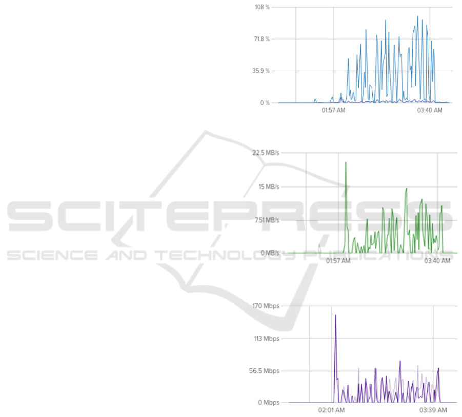
Figure 4: Node CPU load.
Figure 5: Node SSD performance.
Figure 6: Network performance measured in a node.
The Data Warehouse query is presented in
Formula (1). There n=3, m
k
=m
1
. The selectivity of
CD1 was at 67% for the Date table, 90% for Town
table and 80% for Goods. There was no condition
applied to the facts table.
The queries were executed for the following
parameters: the number of slave nodes (N) was 3, 6
IoTBDS 2017 - 2nd International Conference on Internet of Things, Big Data and Security
212

and 9, the number of fact table records (Q
1
) was 10M,
20M and 30M, the Reduce tasks number was 2 and 4.
There were 3(N)·3(Q
1
)·2(s)=18 experiment query (1)
runs on the Data Warehouse. Each query was re-
peated three times and average time was taken. The
measured and modeling time were compared.
The experiments were run on different days for a
different number of nodes. In most cases we observed
high processor load, low disk and network
performance. The Figures 4-6 depict the correspond-
ing characteristics for one node during the execution
of an experiment series for the number of slave nodes
N=6. The number of peaks (equals 18) on each Figure
corresponds to the number of queries in a series for
N=6: 1(N)·3(Q
1
)·2(s)·3(repeat)=18. The processor
core load reached 90%. The shared disk throughput
reached 15MB per second (except a single peak),
while the network throughput reached 60 Mbps.
6.3 Model Calibration and Adequacy
Evaluation
A part of the source data for modeling (N
M
, N
R
, et. al)
was selected from logs generated by Hadoop during
the query execution. For other parameters that cannot
be measured directly we performed a calibration
procedure based on the experiment results. The
following resource performance was evaluated with
the calibration: HDFS (read and write μ
DR
, μ
DW
),
LocalFS (read and write μ
dR
, μ
dW
); switch ports (input
and output μ
PR
, μ
PW
), switch (μ
N1
) and processor
(SLOA time τ). Based on the results of peak
performance measurements we defined the bounda-
ries for these parameters and executed its estimation
with the least squares method (Abdi, 2007). The
Figure 7 provides the estimation algorithm.
An arbitrary selection of the starting point in the outer
loop avoids reaching the local minimum moving
along the gradient.
The following three calibration models were
analyzed:
Option 1. The calibration procedure used the
average time for execution of 6 queries executed on
clusters with 3, 6 and 9 slave nodes. The modeling
accuracy was evaluated for all 18=3(N)·3(Q
1
)·2(s)
queries. The Figure 8 provides the modeling error
distribution diagram. Here
expmodexp
T/T100 T−⋅=Δ
is the relative modeling
error for query execution time by percentage. The
sector on the Figure depicts the fraction of the queries
number (out of 18) which modeling error fits the Δ
half-closed interval. The percentage is shown under
this half-interval. The fraction of queries with
LOOP i= 1…200
Select an arbitrary point inside
calibrated parameter boundaries
LOOP j= 1…200
Move inside the area of calibrated
parameters by gradient (numerical
differentiation is used)
/* The exit from the inner LOOP is performed in the
following 3 cases: 1) if the current sum of error squares
of the average experimental and modeling results for the
query execution time
−=
k
2k
mod
k
exp
)T(T
δ
is
higher than the previous sum (the local minimum is
found); 2) the local calibrated parameter crossed the
measurement boundaries; 3) the j iteration number
exceeds the limit */
END OF LOOP by j
Store the current optimal values for
calibrated parameters
Figure 7: Model parameters calibration algorithm.
modeling error higher than 20% equals to
17+28=45% (this is 18·0.45=8 queries out of 18).
Option 2. The calibration procedure used the
average execution time of four queries executed on
clusters with 6 and 9 slave nodes. The modeling
accuracy was evaluated based on the corresponding
12=2(N)·3(Q
1
)·2(s) queries (i.e. experiments on a
cluster with three slave nodes were excluded). The
Figure 9 provides modeling error distribution
diagram. The fraction of queries with the modeling
error higher than 20% equals to 8% (it is 12·0.08=1
query out of 12).
Option 3. The calibration procedure used the
average time for execution of three queries executed
on the cluster with 9 slave nodes. The modeling
accuracy was evaluated based on the corresponding
6=1(N)·3(Q
1
)·2(s) queries (i.e. experiments on
clusters with 3 and 6 slave nodes were excluded). The
Figure 10 provides the modeling error distribution
diagram. In this case there are no queries with
modeling error higher than 20%.
Figure 8: Modeling error distribution (calibration
Option 1).
Data Warehouse MFRJ Query Execution Model for MapReduce
213

Figure 9: Modeling error distribution (calibration Option 2).
Figure 10: Modeling error distribution (calibration Option
3).
Based on the calibration options 1-3 analysis we
can conclude that the accuracy of the developed
model shows significant growth with the increase in
number of slave nodes in a cluster.
7 CONCLUSION
Based on the performed research we developed an
analytical model that estimates the n-dimensional
Data Warehouse query execution average time for
MapReduce environments with the MFRJ method.
The experiment and modeling results show
that the modeling accuracy grows with the increase in
number of salve nodes. In particular, the error above
20% for 3, 6 and 9 nodes was shown in 8 out of 18
queries. The 9-node runs showed an error rate below
20% for all 6 queries. The demonstrated modeling
accuracy is adequate for the information system
design estimation.
This model checks whether the Data
Warehouse access time is acceptable. This is
especially important for business intelligence systems
with limited response time. The analytical model
application helps a designer to make the right decision
at the right time before the coding is started and well
in advance of the system operation.
The proposed approach can be used for
development of mathematical models for other Data
Warehouse access methods (Zhou & Wang, 2013).
We continue our work on a method for Data
Warehouse with an arbitrary schema (not limited by
the star schema). This method will be based on
cascade application of the Bloom filter and allow
implementing complex SQL queries in the Spark
environment, that cannot be implemented in Hive or
Spark SQL. SELECT operator with a “not equal”
condition applied to a correlated query result is an
example of such complex SQL queries. We work on
a cost model for this method. It will take into account
transformations and operations formed by the query
execution Directed Acyclic Graph and Spark
implementation specifics. A plan can be complex and
represented by an acyclic graph. It works as a
conveyer simultaneously pushing RDD partitions
(table fragments that are stored at the cluster stations)
between the nodes of the graph.
REFERENCES
Abdi, H. (2007) The method of least squares. In N. Salkind,
editor, Encyclopedia of Measurement and Statistics.
CA, USA: Thousand Oaks.
Afrati, F. N. , Sarma, A. D., Salihoglu, S. and Ullman, J. D.
(2012) Upper and lower bounds on the cost of a map-
reduce computation. CoRR, abs/1206.4377,
Proceedings of the VLDB Endowment, Volume 6
Issue 4, February 2013, Pages 277-288, ACM New
York, NY, USA.
Afrati, F.N. and Ullman, J.D. (2010) Optimizing joins in a
map-reduce environment. In Proceedings of the 13th
International Conference on Extending Database
Technology, ACM New York, NY, USA.
Burdakov, A.V., Grigorev, U.A., Ploutenko, A.D. (2014)
Comparison of table join execution time for parallel
DBMS and MapReduce, Software Engineering / 811:
Parallel and Distributed Computing and Networks /
816: Artificial Intelligence and Applications
Proceedings (March 18 – 18, 2014, Innsbruck, Austria),
ACTA Press, 2014.
Digital Ocean (2016), Available: www.digitalocean.com,
[21 February 2017].
Duda, J. (2012) Business intelligence and NoSQL
databases. Information Systems in Management
(2012), Vol. 1 (1), pp. 25-37.
Golfarelli, M. and Rizzi, S. (2009) Data Warehouse
Design: Modern Principles and Methodologies.
McGraw-Hill, Inc. New York, NY, USA. P. 458.
Hejmalíček, B. A. (2015) Hadoop as an Extension of the
Enterprise Data Warehouse. Masaryk university,
Faculty of informatics, Brno, Czech Republic.
Huai, Y., Chauhan, A., Gates, A. et al. (2014) Major
Technical Advancements in Apache Hive, SIGMOD '14
IoTBDS 2017 - 2nd International Conference on Internet of Things, Big Data and Security
214

Proceedings of the 2014 ACM SIGMOD International
Conference on Management of Data, pages 1235-1246,
ACM, New York, NY, USA.
Inmon, W. H. (2005) Building the Data Warehouse, Fourth
Edition. Wiley Publishing, Inc. P. 576, Indianapolis, IN,
USA.
Jeffrey Dean, Sanjay Ghemawat (2004). MapReduce:
Simplified Data Processing on Large Clusters. Sixth
Symposium on Operating System Design and
Implementation (OSDI’04), San Francisco, CA, USA.
Karloff, H., Suri, S. and Vassilvitskii S. (2010) A model of
computation for MapReduce. In Proceedings of the
Twenty-First Annual ACM-SIAM Symposium on
Discrete Algorithms, SODA ’10, pages 938–948,
Philadelphia, PA, USA, 2010. Society for Industrial and
Applied Mathematics.
Kaur, A. (2016) Big Data: A Review of Challenges, Tools
and Techniques. International Journal of Scientific
Research in Science, Engineering and Technology
(IJSRSET), Volume 2, Issue 2, pp. 1090-1093,
TechnoScience Academy.
Koutris, P. and Suciu, D. (2011) Parallel evaluation of
conjunctive queries. In Proceedings of the 30th ACM
SIGACT-SIGMOD-SIGART Symposium on
Principles of Database Systems. ACM, New York, NY,
USA, 223–234.
Li, B., Mazur, E., Diao, Y., McGregor, A. and Shenoy, P.J.
(2011) A platform for scalable one-pass analytics using
MapReduce. In: Proceedings of the ACM SIGMOD
International Conference on Management of Data
(SIGMOD), pp. 985–996, ACM, New York, NY, USA.
Li, F., Ooi, B. C., Özsu, M. T., Wu, S. (2014) Distributed
data management using MapReduce. Journal ACM
Computing Surveys (CSUR), Volume 46, Issue 3,
January 2014, Article No. 31, ACM, New York, NY,
USA.
Palla, K. (2009) A comparative analysis of join algorithms
using the Hadoop Map/Reduce framework. Master’s
Thesis, University of Edinburgh, Edinburgh, UK.
Available:www.inf.ed.ac.uk/publications/thesis/online/
IM090720.pdf, [21 February 2017].
Pavlo, A., Paulson, E., Rasin, A., Abadi, D.J., DeWitt, D.J.,
Madden, S.R. and Stonebraker, M.A. (2009) A
comparison of approaches to large-scale data analysis.
In Proceedings of the 35th SIGMOD International
Conference on Management of Data. ACM Press, New
York, 165–178.
Redmond, E. and Wilson, J.R. (2012) Seven Databases in
Seven Weeks: A Guide to Modern Databases and the
NoSQL Movement. Pragmatic Bookshelf, Pragmatic
Programmers, USA.
Sadalage, P. and Fowler, M. (2012) NoSQL Distilled: A
Brief Guide to the Emerging World of Polyglot
Persistence. Addison Wesley Professional,
Crawfordsville, IN, USA.
Simhadri, H. V. (2013) Program-Centric Cost Models for
Locality and Parallelism. PhD thesis, Carnegie Mellon
University (CMU). Pittsburgh, PA, USA. Available:
www.cs.cmu.edu/~hsimhadr/thesis.pdf, [21 February
2017].
Tao, Y., Lin, W., and Xiao, X. (2013) Minimal mapreduce
algorithms. In Proceedings of the 2013 ACM SIGMOD
International Conference on Management of Data,
SIGMOD ’13, pages 529–540, New York, NY, USA.
ACM.
White, T. (2015) Hadoop: The Definitive Guide, 4th
Edition. O'Reilly Media, Sebastopol, CA, USA.
Wu, S., LI, F., Mehrotra, S. and Ooi, B.C. (2011) Query
optimization for massively parallel data processing. In
Proc. 2nd ACM Symposium on Cloud Computing.
12:1–12:13. ACM, New York, NY, USA.
Zhou, G. Z. and Wang, G. Y. (2013) Cache Conscious Star-
Join in MapReduce Environments. Cloud-I '13
Proceedings of the International Workshop on Cloud
Intelligence, Riva del Garda, Trento, Italy — August
26-26, 2013, ACM New York, NY, USA.
Data Warehouse MFRJ Query Execution Model for MapReduce
215
