
Cell Trajectory Clustering: Towards the Automated Identification of
Morphogenetic Fields in Animal Embryogenesis
Juan Raphael Diaz Simões
1,2
, Paul Bourgine
1,3
, Denis Grebenkov
2
and Nadine Peyriéras
1
1
BioEmergences USR3695, CNRS, Université Paris-Saclay, 91198 Gif-sur-Yvette Cedex, France
2
CNRS, Université Paris-Saclay, Route de Saclay, 92128 Palaiseau Cedex, France
3
Complex Systems Institute Paris Île-de-France UPS3611, CNRS, 113 rue Nationale, 75013 Paris, France
Keywords:
Animal Embryogenesis, Cell Lineage, Clustering, Path Integrals.
Abstract:
The recent availability of complete cell lineages from live imaging data opens the way to novel methodologies
for the automated analysis of cell dynamics in animal embryogenesis. We propose a method for the calcula-
tion of measure-based dissimilarities between cells. These dissimilarity measures allow the use of clustering
algorithms for the inference of time-persistent patterns. The method is applied to the digital cell lineages
reconstructed from live zebrafish embryos imaged from 6 to 13 hours post fertilization. We show that the
position and velocity of cells are sufficient to identify relevant morphological features including bilateral sym-
metry and coherent cell domains. The method is flexible enough to readily integrate larger sets of measures
opening the way to the automated identification of morphogenetic fields.
1 INTRODUCTION
Embryogenesis involves the formation of boundaries
between cell populations, which leads to the individu-
ation of cell compartments (Fagotto, 2014). Cells gat-
hered in the same compartment are expected to have
behavioral similarities, depending on the animal spe-
cies and the spatio temporal morphogenetic sequence.
The formation of morphogenetic fields and compart-
ments being a progressive phenomenon, similarities
in cell behaviors should be present at early stages.
Furthermore, behavioral similarities should be passed
from mother to daughters along the cell lineage.
In this context, the proposed similarity (or dissimi-
larity) measure of cell behavior should have the follo-
wing properties:
• It should be flexible enough to deal with different
sets of measures, different animal species and dif-
ferent periods of the organism development.
• It should consider the cell as a structure with a
temporal coherence.
• It should take into account the relative persistence
of cell characteristics along their lineage.
We propose a method to measure dissimilarities
between cells based on their behaviors along the cell
lineage. The dissimilarity calculation method is in-
spired from path integrals in quantum mechanics and
stochastic processes (Feynman, 1965) and is valid for
measures taken at the level of single cells throughout
the duration of their cell cycle.
This measure is further used for the automatic
clustering of cell trajectories.
The method is applied to the analysis of digital
cell lineage trees reconstructed from live zebrafish
embryos imaged in 3D+time. We show that a mi-
nimal set of parameters can lead to clusters highlig-
hting morphogenetic features from the organism bi-
lateral symmetry to finer cellular domains consistent
with the cell compartments that shape the presump-
tive organs.
2 ALGORITHM DESCRIPTION
The algorithm can be decomposed into the following
steps:
1. Extracting measures from input data. In the
case presented here, the data consisted in the
cell lineage reconstructed from partial 3D+time
imaging of developing zebrafish embryos (Faure
et al., 2016). The digital cell lineage provides the
cell positions in space and time. Velocities are cal-
culated using a discrete derivative similar to low-
pass filters (Holoborodko, 2008). This choice is
justified by the fact that the noise on the trajecto-
ries is unknown;
746
Simões, J., Bourgine, P., Grebenkov, D. and Peyriéras, N.
Cell Trajectory Clustering: Towards the Automated Identification of Morphogenetic Fields in Animal Embryogenesis.
DOI: 10.5220/0006259407460752
In Proceedings of the 6th International Conference on Pattern Recognition Applications and Methods (ICPRAM 2017), pages 746-752
ISBN: 978-989-758-222-6
Copyright
c
2017 by SCITEPRESS – Science and Technology Publications, Lda. All rights reserved

2. Calculating the genealogic dissimilarities bet-
ween cell trajectories. This step is described in
detail in the following sections;
3. Using these dissimilarities as input for a cluste-
ring algorithm. We used spectral clustering (Ng
et al., 2001) since it is easy to implement, efficient
enough to allow the test of parameters and works
with sparse dissimilarity matrices (von Luxburg,
2007).
In the following sections we present the steps for
the calculation of genealogic dissimilarities, comment
on some practical aspects of parameters and efficiency
and discuss the results. The overall methodology is
schematized in Fig. 1.
3 TRAJECTORIES,
GENEALOGIES AND
DISSIMILARITIES
The data sets used here are partial, since the mi-
croscope images only cover a limited region of the
embryo. This leads to the following division of a cell
lifetime. We define the lifetime of a cell as the inter-
val of time between its birth at the time of it’s mot-
her’s division or its entrance into the field of view and
its division or exit from the field of view. From this
definition mother cells and daughters are different en-
tities, connected by the cell lineage.
In addition, cells can only be compared at the
same point in time as their behavior changes du-
ring the embryogenesis. Our algorithm is made to
overcome this difficulty and compare cell behaviors
throughout an entire relevant developmental period by
extending the cell lifetime period by that of its pro-
geny through a probabilistic approach.
3.1 Defining Cell Rajectories
Given a totally ordered time set T, which may be dis-
crete or continuous, and a state set S of measures,
we define a trajectory to be a dependent tuple (I,x),
where I =]I
−
,I
+
] is an interval in T and x : I → S is
a function into the state space. We call the space of
trajectories in time T and state S by T (T,S).
3.2 An Algebra for Trajectories
The calculation of dissimilarities between trajectories
involve the intersection and concatenation of trajecto-
ries, the fundamental operations of the method. Ho-
wever, because it’s not true that every pair of cells
share a point in time where they coexist, we will need
to introduce the notion of undefined values to deal
with these cases.
We define a possibly undefined value of type X to
be an element of the set X = X ∪ {U} where the unde-
fined value U has been added. Any function f : X → Y
can be lifted to a function f : X → Y by
f (U) = U
f (x) = f (x)
We use X = (I,x) and Y = (J,y) as example tra-
jectories. We define trajectory concatenation ∨ for
trajectories satisfying I
+
= J
−
by
X ∨Y = (I ∪ J,x ∨ y)
where
[x ∨ y](t) =
(
t ∈ I ⇒ x(t)
t ∈ J ⇒ y(t)
This operation can be lifted to T (T,S), by making
U a unity
X∨Y =
X = U ⇒ Y
Y = U ⇒ X
otherwise ⇒ X ∨Y
We define moreover trajectory intersection ∧ :
T (T,S) × T (T,S) → T (T,S
2
) by
X ∧Y =
(
I ∩ J 6=
/
0 ⇒ (I ∩ J, (x, y)|
I∩J
)
otherwise ⇒ U
An example is shown in Fig. 2. This operation can be
lifted to T (T,S) by defining U to be a zero
X∧Y =
X = U ⇒ U
Y = U ⇒ U
otherwise ⇒ X ∧Y
With these definitions, it is not hard to prove the
distributivity of intersection over concatenation
Z∧(X∨Y) = (Z∧X)∨(Z∧Y ) (1)
In the following sections, we will always write ∧
and ∨ instead of ∧ and ∨ for easier reading, but all
operations are defined with relation to the later.
3.3 Genealogic Trajectories
A genealogic trajectory is a cell trajectory that has
been extended probabilistically by the trajectories of
its progeny. The definition is recursive. For any tra-
jectory X we define i
X
as an equiprobable zero-one
random variable. The genealogical trajectory
e
X is a
trajectory-valued random variable such that
Cell Trajectory Clustering: Towards the Automated Identification of Morphogenetic Fields in Animal Embryogenesis
747
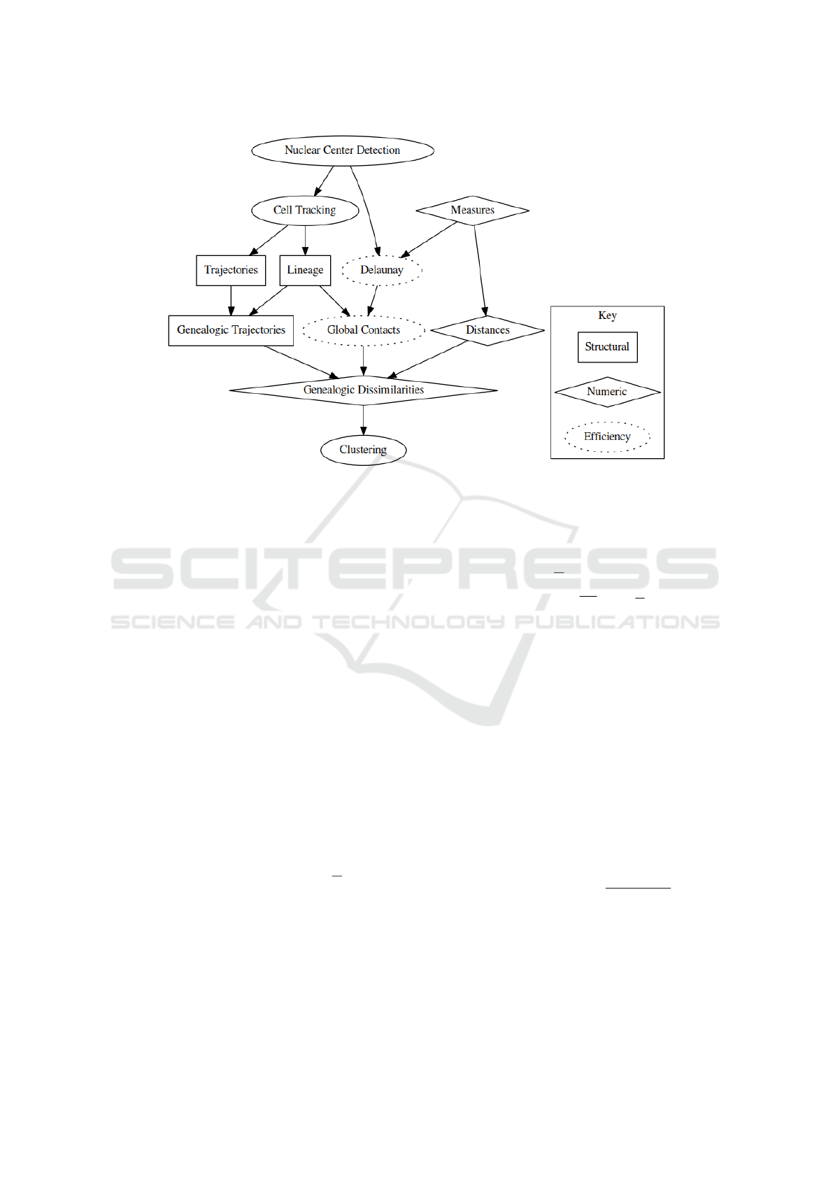
Figure 1: Scheme describing the steps of the algorithm. In square boxes are the steps necessary for the construction of
the structural entities: the cell lineage and genealogical trajectories. In diamond-shaped boxes are the numerical entities,
corresponding to measures, in this case position and velocity and the corresponding distances and dissimilarities. In dotted
boxes are the entities necessary for the efficient calculation of the clustering, namely the definition of neighboring cells.
1. If X has no siblings,
e
X = X;
2. If X has siblings Y
0
and Y
1
then
e
X = X ∨
e
Y
i
X
.
An example is shown in Fig. 2. Moreover, if X 6=
Y then i
X
and i
Y
assumed to be independent. This
allows the simple calculation of expectations.
3.4 Dissimilarities and Weights
A dissimilarity in S is a symmetric positive function
d : S × S → R. Given the two trajectories X = (I, x)
and Y = (J, y), X ∧ Y = (K,z), a dissimilarity d in S
and a measure µ in T, we define the partial dissimila-
rity P
µ,d
between two trajectories as
P
µ,d
(X,Y ) =
µ(K),
Z
K
d ◦ zdµ
The set R
2
has a natural monoidal structure given
by the sum of coordinates represented by ⊕. By gi-
ving the following monoidal structure to R
2
a ⊕ b =
a = U ⇒ b
b = U ⇒ a
otherwise ⇒ a ⊕ b
We can prove that P
µ,d
satisfies the following
P
µ,d
(X ∨Y) = P
µ,d
(X)⊕ P
µ,d
(Y) (2)
Finally, we define the dissimilarity D
µ,d
:
T (T,S) × T (T,S) → R as
D
µ,d
(X,Y ) = divP
µ,d
(X∧Y )
where div(m, s) = s/m, considering 0/0 = U.
The genealogical dissimilarity between two tra-
jectories is defined as
e
D(X,Y ) = E[D(
e
X,
e
Y)] (3)
where E denotes expectation. This definition is ana-
logous to path integrals in quantum mechanics.
Equation (2) gives a way to decompose genealo-
gical dissimilarities into regular dissimilarities, mea-
ning that genealogical dissimilarities can be calcula-
ted from the matrix of pairwise partial dissimilarities
P
µ,d
(Z ∧ (X ∨Y)) = P
µ,d
(Z ∧ X) ⊕ P
µ,d
(Z ∧Y )
Finally, we define the similarity S
µ,d,σ
: T (T, S) ×
T (T,S) → R as
S
µ,d,σ
(X,Y ) = exp
"
−
e
D
µ,d
(X,Y )
2
2σ
2
#
(4)
where σ is a scale factor.
3.5 Properties
Let us consider a simple lineage with a cell M, two
daughters C
1
and C
2
and a cell N with no daughters.
ICPRAM 2017 - 6th International Conference on Pattern Recognition Applications and Methods
748
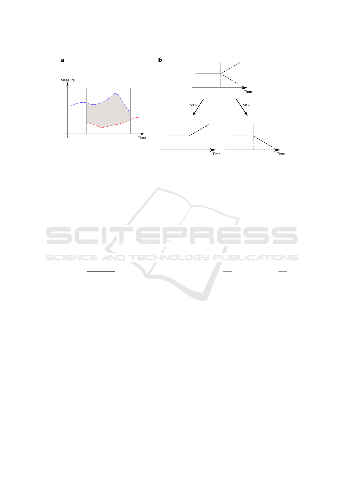
Figure 2: a Intersection of the trajectories of two cells (red and blue) represented in an abstract measure space. The starting
point of each cell trajectory can be due to either cellular division of the mother or entrance of the cell into the imaging field of
view. It may also result from artefacts of the tracking algorithm. Similarly, the ending point of each cell trajectory corresponds
either its division, its exit out of the imaging field of view or to tracking errors. Only the difference of measures (grey) inside
this interval are taken into account. b A schematic cell lineage with the lifetime if a mother cell (continuous line) and the
lifetime of its two daughters (dashed lines). The probabilistic transformation of the mother history gives rise to two different
paths with equal probabilities. This process is done recursively throughout consecutive cell divisions along the cell lineage.
If M and N do not coexist at any point in time, formula
(1) states
e
D
µ,d
(M,N) =
e
D
µ,d
(C
1
,N) +
e
D
µ,d
(C
2
,N)
2
In particular
e
D
µ,d
(M,C
1
) =
e
D
µ,d
(C
1
,C
2
)
2
=
e
D
µ,d
(M,C
2
) (5)
This equation shows that the mother is equidistant
to its daughters and that if both daughters stay close
to each other, their mother stays close to both of them,
leading to a degree of coherence between their cluste-
ring allocations.
Another important property is given by the appli-
cation of equation (2), adding a point in time for Z.
This can be written as
P
µ,d
(X ∧(Z ∨ Z
0
)) = P
µ,d
(X ∧Z) ⊕P
µ,d
(X ∧Z
0
)
meaning that the partial dissimilarity can be processed
incrementally in time.
3.6 Definition of Similarities
If the state space has the form
∏
k
S
k
, where each coor-
dinate has a corresponding dissimilarity d
k
, any term
of the form
d
λ
=
∑
k
λ
k
d
k
is also a dissimilarity on S, where every λ
k
> 0. If s
k
is the similarity associated to d
k
then
s
λ
=
∑
k
λ
k
s
k
is also a similarity and this is the definition used in this
article. In the case of two dissimilarities that gives:
s
λ
= λ exp
−
d
2
1
2σ
2
1
+ (1 − λ)exp
−
d
2
2
2σ
2
1
In order to have a good equilibrium between similari-
ties, we choose σ
k
to be equal to the standard devia-
tion of d
k
.
4 COMPUTATIONAL
EFFICIENCY
Following the regular clustering algorithm, we need
to provide the whole similarity matrix, which gives
a complexity of O(n
2
) on the number of trajectories.
Moreover, because the matrix is dense, extracting a
even few eigenpairs from it is very costly.
A common method of simplification is to use only
the few largest similarities, making the matrix sparse
and its largests eigenvectors fast to calculate. Howe-
ver, the whole matrix still has to be calculated.
We propose an alternative simplification by cal-
culating the similarities between neighbor trajectories
only. Two trajectories are considered neighbors if
Cell Trajectory Clustering: Towards the Automated Identification of Morphogenetic Fields in Animal Embryogenesis
749
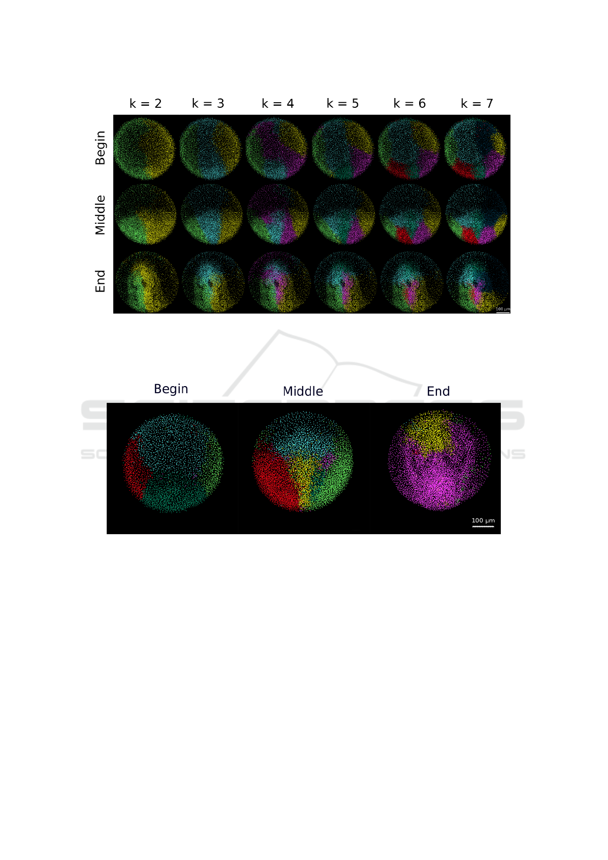
Figure 3: Patterns defined by the clustering algorithm Processing of the dataset 141108aF with λ = 0.5. 3D rendering of
the embryo displayed with dots corresponding to detected nuclei. The different clusters are distinguished by their color chosen
arbitrarily. The chosen number of clusters varies from 2 to 7 displayed in the different columns. The embryo is observed from
the animal pole, anterior to the top at 6h54 (Begin - first row), 9h31 (Middle - second row) and 12h10 hpf (End - third row).
Scale bar 100 µm.
Figure 4: Example of the artifact of temporal variability of the segmentation patterns Processing of dataset 071226a
with λ = 0.5 and k = 6. 3D rendering as in Figure 3. The embryo is observed from the animal pole, anterior to the top from
6h54 (begin), 9h31 (middle) and 12h10 hpf (end). Scale bar 100 µm. The flow of cells into and out of the imaged volume
breaks the coherence of the cell lineage and consequently the spatial and temporal coherence of the patterns identified by our
method.
they are neighbors one time step at least, in either po-
sition of velocity (or any other chosen euclidean me-
asure). The concept of neighborhood is based on the
Delaunay tesselation performed at each time step and
for every measure.
A typical data set encompassing zebrafish em-
bryonic development from 6hpf to 13 hpf imaged
from the animal pole (Faure et al., 2016) has around
350 time steps, 6000 cells per time step and altoget-
her 100000 cell trajectories. Given these numbers, the
tradeoff between the complexity added by the tesse-
lation at each time step and a global dense matrix is
very positive. The original algorithm would process
only very small data sets, while the improved version
processes typical data sets within a few hours on a
standard desktop computer.
ICPRAM 2017 - 6th International Conference on Pattern Recognition Applications and Methods
750
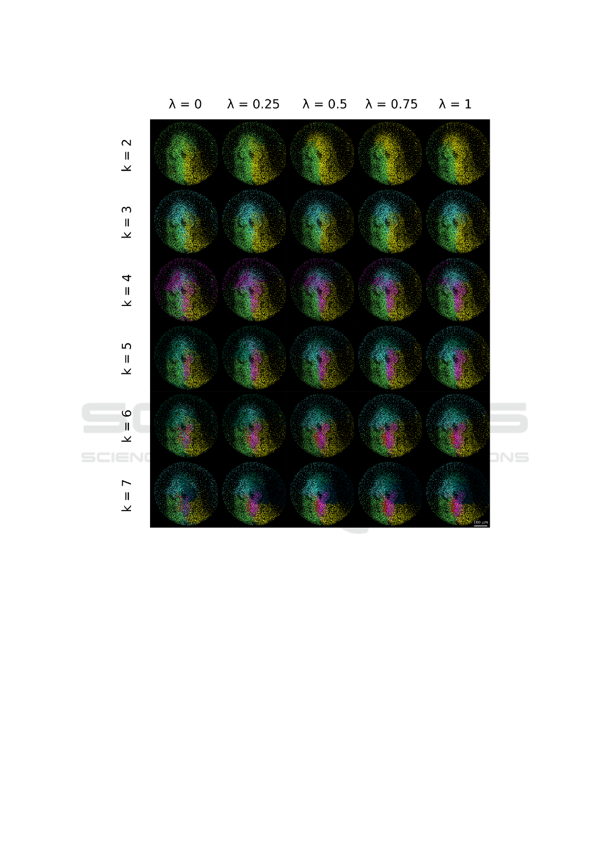
Figure 5: Parameter space exploration for the specimen 141108aF. The patterns obtained with the clustering algorithm
when varying λ and k are displayed. Each row corresponds to the chosen number of clusters varying from 2 to 7. Different
values of λ corresponding to the relative weight of cell position and velocity are displayed in columns, with the relative weight
of position increasing from left to right.
5 RESULTS : APPLICATION TO
ZEBRAFISH DIGITAL
LINEAGE TREES
The relevance of the method to the analyzis of digital
cell lineage trees has been assessed on two datasets
corresponding to wild type zebrafish embryos iden-
tified as 141108aF and 071226a, developing over 8
hours encompassing gastrulation stages. These de-
tails have been described in detail in (Faure et al.,
2016). The application of our algorithm to 141108aF
(Fig. 3) shows that for a number of clusters equal
to 2, the embryo is segmented through its bilateral
symmetry plane. This appears as an interesting emer-
ging feature, not being imposed at all by the method.
Furthermore, when increasing the number of clusters,
embryonic tissues are segmented in visually coherent
domains.
The results of the algorithm are very sensitive to
the persistence of cells inside the imaged volume, as
shown by the results for 071226a (Fig. 4). As the
imaged volume encompasses only the animal top of
the embryo, there is an extensive flow of cells into
Cell Trajectory Clustering: Towards the Automated Identification of Morphogenetic Fields in Animal Embryogenesis
751

and out of the imaged volume that creates a temporal
segmentation that blurs the coherence the spatial or-
ganization that we expect to characterize. This limita-
tion comes from the data, not from the algorithm, and
would be solved if the data encompassed the whole
embryo. Artifacts due to the incompleteness of the
imaging data also compromise the possibility to quan-
tify interindividual differences.
The algorithm can be tuned by exploring the para-
meter space defined by λ and k (Fig. 5), λ correspon-
ding to the relative weight given to the different mea-
sures and k to the number of clusters. We observed, as
expected, that privileging cell position over cell velo-
city led to more compact patterns and domains with
sharper boundaries.
6 CONCLUSION
Our algorithm for measuring cell behavior similarity
based on cells’ trajectory clustering takes into account
an arbitrary number of measures derived from digi-
tal cell lineage trees and translates them into coherent
cell groups.
The major limit identified in the study come from
the incompleteness of the imaging data. It should ho-
wever be noted that taking into account an even larger
number of cells would bring other difficulties.
The results that reveal coherent domains based on
cell behavior similarity are meaningful for the biolo-
gist as they automatically reveal morphological land-
marks. A next step will be to systematically compare
the obtained patterns with patterns defined otherwise,
such as gene expression patterns or fate maps. Our
algorithm is expected to be a valuable addition to the
growing toolbox for algorithmically augmented ob-
servation and the analysis of animal embryonic mor-
phogenesis, opening new paths of research.
REFERENCES
Fagotto, F. (2014). The cellular basis of tissue separation.
Development 141, 3303-3318.
Faure, E. et al. (2016). A workflow to process 3d+time mi-
croscopy images of developing organisms and recon-
struct their cell lineage. Nature Communications 2016
25 Feb; 7:8674.
Feynman, R. P.; Hibbs, A. R. (1965). Quantum Mechanics
and Path Integrals. New York: McGraw-Hill.
Holoborodko, P. (2008). Smooth noise robust differentia-
tors. http://www.holoborodko.com/ pavel/numerical-
methods/numerical-derivative/smooth-low-noise-
differentiators/.
Ng, A. Y., Jordan, M. I., and Weiss, Y. (2001). On spectral
clustering: Analysis and an algorithm. In Advances In
Neural Information Processing Systems, pages 849–
856. MIT Press.
von Luxburg, U. (2007). A tutorial on spectral clustering.
Statistics and Computing, 17 (4).
ICPRAM 2017 - 6th International Conference on Pattern Recognition Applications and Methods
752
