
Reference Plane based Fisheye Stereo Epipolar Rectification
Nobuyuki Kita and Yasuyo Kita
Intelligent Systems Research Institute, National Institute of Advanced Industrial Science and Technology (AIST),
Tsukuba Central 1, Tsukuba 305-8560, Japan
{n.kita, y.kita}@aist.go.jp
Keywords: Fisheye Stereo, Epipolar Rectification, Stereo Measurement, Humanoid Robot, Multi Contact, Near Support
Plane.
Abstract: When a humanoid robot walks through or performs a task in a very narrow space, it sometimes touches the
environment with its hand or arm to retain its balance. To do this the robot must identify a flat surface of
appropriate size with which it can make sufficient contact; the surface must also be within reach of robot's
upper body. Using fisheye stereo vision, it is possible to obtain image information for a field of view wider
than that of a hemisphere whose central axis is the optical axes; thus, three dimensional distances to the
possible contact spaces can be evaluated at a glance. To realize it, stereo correspondence is crucial.
However, the short distance between the stereo cameras and the target space causes differences in the
apparent shapes of the targets in the left and right images, which can make stereo correspondence difficult.
Therefore, we propose a novel method which rectifies stereo images so that the targets have the same
apparent shapes in the left and right images when the targets are close to a reference plane. Actual fisheye
stereo image pairs were rectified, and three dimensional measurements were performed. Better results were
obtained using the proposed rectification method than using other rectification methods.
1 INTRODUCTION
Humanoid robots are expected to substitute or
support the work of humans in many places such as
at disaster sites, airplane assembly plants, and
building sites. As such, humanoid robots must be
able to traverse narrow spaces and conduct tasks that
require their upper body parts, e.g., hands, elbows,
and shoulders, in addition to the soles of their feet to
maintain their balance (Sentis, 2010), (Escande,
2013), (Henze, 2016). To realize such stabilization
motions in unknown environments, a planar area
which has proper sizes and poses have to be
identified in the vicinity of the humanoid robot's
upper body (Brossette, 2013), (Khatib, 2014). The
measurements that are necessary to adequately
evaluate the environment are as follows.
1. Dense three dimensional (3D) distance
measurements.
2. 3D distance measurements in reach of the robot.
3. 3D distance measurements of the immediate
vicinity of the humanoid robot's upper body.
4. Fast 3D distance measurements.
5. 3D distance measurements of poorly textured
surfaces.
Various types of equipment have been developed
for 3D distance measurements. The most popular is
the RGB-D sensor (where the D represents the
"depth" channel); this sensor can perform
measurements 1, 4, and 5. Measurement 3 can be
achieved by controlling the pose of a sensor.
However, there are no off-the-shelf RGB-D sensors
that can perform measurement 2. Most teams that
signed-up for the DRC (Defense Advanced Research
Projects Agency Robotics Challenge) in 2015 used a
spinning LIDAR sensor, which is high-speed
rotational 1D scanning type LRF (Laser rangefinder).
This type of sensor can conduct measurements 1, 3,
4, and 5. However, the closest distance at which
LRFs work is 0.5 m, which is too far to enable
measurement 2 to be conducted. For a long time
now, stereo vision that uses multiple cameras has
been used for 3D distance measurements. There are
numerous studies on stereo measurements and many
available products. However, the width of the space
these products can measure is limited because they
usually use cameras with normal fields of view; thus,
additional pose control equipment is necessary to
carry out measurement 3.
308
Kita N. and Kita Y.
Reference Plane based Fisheye Stereo Epipolar Rectification.
DOI: 10.5220/0006261003080320
In Proceedings of the 12th International Joint Conference on Computer Vision, Imaging and Computer Graphics Theory and Applications (VISIGRAPP 2017), pages 308-320
ISBN: 978-989-758-227-1
Copyright
c
2017 by SCITEPRESS – Science and Technology Publications, Lda. All rights reserved
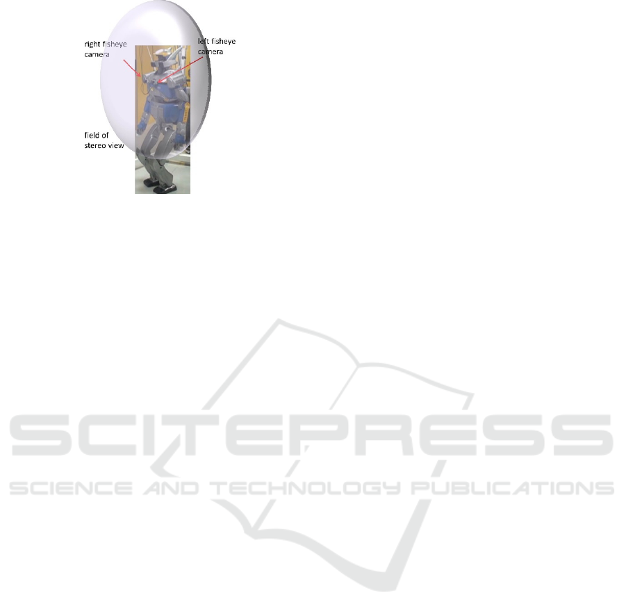
Figure 1: Humanoid robot with fisheye stereo.
Some fisheye lenses have wide fields of view
(larger than 180°). Mounting two cameras equipped
with such fisheye lenses in parallel on the chest of a
humanoid robot yields a stereo field of view greater
than 180° with an optical axis that is in the forward
direction, as shown in Figure 1. For stereo
measurements, stereo correspondence is crucial.
However, the distance from the stereo cameras to the
target space is short compared with the baseline
length of the stereo system; this causes differences
in the apparent shapes of the targets in the left and
right images. Furthermore, some targets have no
clear visual features, which makes stereo
correspondence difficult. In this paper, we propose a
novel method that rectifies stereo images so that the
targets have the same apparent shapes in the left and
right images when the targets reside close to a
reference plane.
In Section 2 of this paper, we introduce related
stereo vision studies and background information
related to the proposed method is presented. In
Section 3, the proposed rectification method, which
is based on a reference plane, is explained. In
Section 4, we present the rectification of actual
fisheye stereo image pairs using the proposed
method by changing the pose of the reference plane
while three dimensional measurements are
performed using a simple region-based matching
method. The experimental results show that using
the proposed rectification method yields better
results than using other rectification methods when
the reference plane is close to the actual target.
Finally, in Section 5 we summarize our work and
discuss potential future research ideas.
2 RELATED WORKS
In the above section, the necessary measurements to
sufficiently evaluate the environment in the
immediate vicinity of a robot were detailed. Based
on those, there are some conditions that make it
difficult to conduct stereo measurements.
D1. The targets are too close (i.e., the distance from
the robot is between one to several times that
of the stereo baseline length).
D2. The texture of targets is sometimes poor.
D3. The target may lie on an extension of the stereo
baseline.
When the target is close to the stereo cameras, its
appearance differs greatly between the left and the
right image. Similar problems occur even for wide
baseline stereo systems, and many methods have
been proposed to tackle these problems (Schmid,
1997), (Baumberg, 2000), (Matas, 2004), (Bay,
2005). Most such methods first detect salient
features and then derive descriptions that are
invariant of the viewing direction. Then the
correspondences are taken based on the measure of
similarity of the descriptions. The existing methods
are not suitable for a target that has no clear visual
features.
For a poorly textured target, most methods derive
a local description from the intensity changes in the
local region and then take correspondences based on
the similarity measure of those descriptions
(Scharstein, 2002). Several important approaches
have been proposed for such region-based methods.
Epipolar constraint
Rectification
Cost function
If the stereo parameters are known, the search region
can be constrained on an epipolar line to reduce the
risk of mismatching (Hartley, 2003). Further, the left
and right images are often transformed so that the
epipolar lines coincide with the image rows via
rectification (Ayache, 1988), (Courtney, 1992),
(Loop, 1999), (Hartley, 1999). Various cost
functions have been developed to determine a
measure of similarity for local regions (Hirschmuller,
2009). The simplest ones directly utilize the local
regions' intensities, e.g., the sum of squared
difference (SSD) and normalized SSD (NSSD)
functions. Some functions compare descriptors that
are derived from the images filtered using Sobel
operator, Gauss operator, or other operators (Zabih,
1994), (Geiger, 2010). Complicated functions have
primarily been developed to cope with differences in
the brightness between the left and right images
(Hirschmuller, 2008). Few methods have been
developed to handle differences in the apparent
shape of objects between the left and right images
(Devernay, 1994), (Tola, 2010).
Reference Plane based Fisheye Stereo Epipolar Rectification
309
One stereo vision method measures the ragged
shape of a ground surface using a fisheye stereo
system (Kita, 2011). First a rectification method is
used that transforms only the ground portion of the
images so that the disparity becomes zero on the
expected ground plane. Because the differences in
the apparent shapes in the left and right images
become small around the ground plane,
correspondences can be obtained using simple cost
functions even when the texture is poor. This
method seems to solve the difficulties D1 and D2.
But unfortunately, the rectification method used in
that method does not work when the measurement
target lies on an extension of the stereo baseline.
Pollefeys used a polar coordinate system to
rectify two images that were obtained before and
after the camera was moved forward to include two
epipoles (Pollefeys, 1999). Abraham also used a
polar coordinate system to rectify stereo images that
were obtained by two parallel cameras mounted with
fisheye lenses (Abraham, 2005). Difficulty D3 can
be overcome by using a polar coordinate system, but
both methods mentioned above were not conceived
to cope with the differences in apparent shape
between the left and right images.
In this paper, we therefore propose a new
rectification method that combines the approach of
achieving zero disparity on a reference plane and the
approach of using a polar coordinate system. The
advantages of the proposed method are as follows.
It enables a reference plane to be set on an
extension of the stereo baseline.
Because the differences of the apparent shapes
on the left and right images become small for a
target that is close to the reference plane,
correspondences can be obtained using simple
cost functions, even when the texture is poor.
3 REFERENCE PLANE BASED
RECTIFICATION METHOD
The proposed method rectifies only a portion of the
fisheye images so that the disparity becomes zero on
a reference plane. Because something on the
reference plane shows the same apparent shape in
the left and right rectified images, the
correspondence can be detected using a simple
region-based matching method with high reliability.
Though the reference plane was set manually in the
experiments presented in Section 4, in practice it
would be set by the humanoid robot at an area that a
part of its upper body, e.g., hand, may come in
contact with to help it maintain its balance. In the
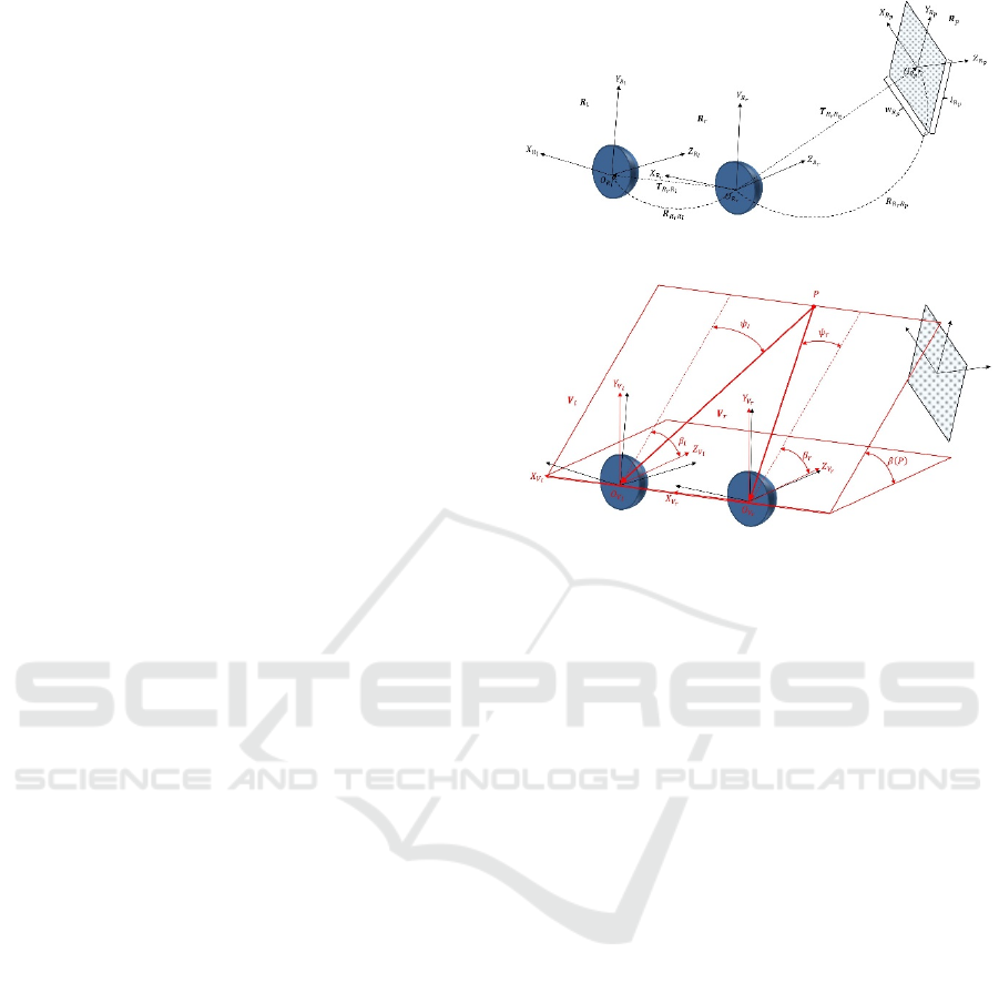
Figure 2: Coordinate frames.
Figure 3: Virtual camera coordinate frames.
latter part of this section, some coordinate frames are
first defined, the method for deciding which part of
the fisheye images should be rectified is explained,
and finally the method to transform the fisheye
images to rectified images is introduced.
3.1 Coordinate Frames
Figure 2 shows left and right fisheye camera
coordinates,
and
. Here, for simplicity,
is a
base frame instead of the world frame. The origins
are the optical centers, the Z axes are the optical axes,
and the Y axes are the upper directions of the images
(for simplicity, we assume that the image plane is
perpendicular to the optical axis). The pose of
is
represented by the translation
and the rotation
, which are assumed to be calibrated in
advance. Figure 2 depicts the reference plane. It is a
rectangle of size
. A coordinate frame
is
defined as shown in Figure 2. The origin is the
center of the rectangle, the Y axis is the length
direction, the X axis is the width direction, and the Z
axis is the normal direction of the backside of the
reference plane. The pose of the reference plane is
set by the translation
and the rotation
.
Because the cameras must be aligned in parallel
to generate the rectified images (Figure 3), the
virtual camera coordinate frames,
and
, are
defined as follows (Figure 3).
VISAPP 2017 - International Conference on Computer Vision Theory and Applications
310
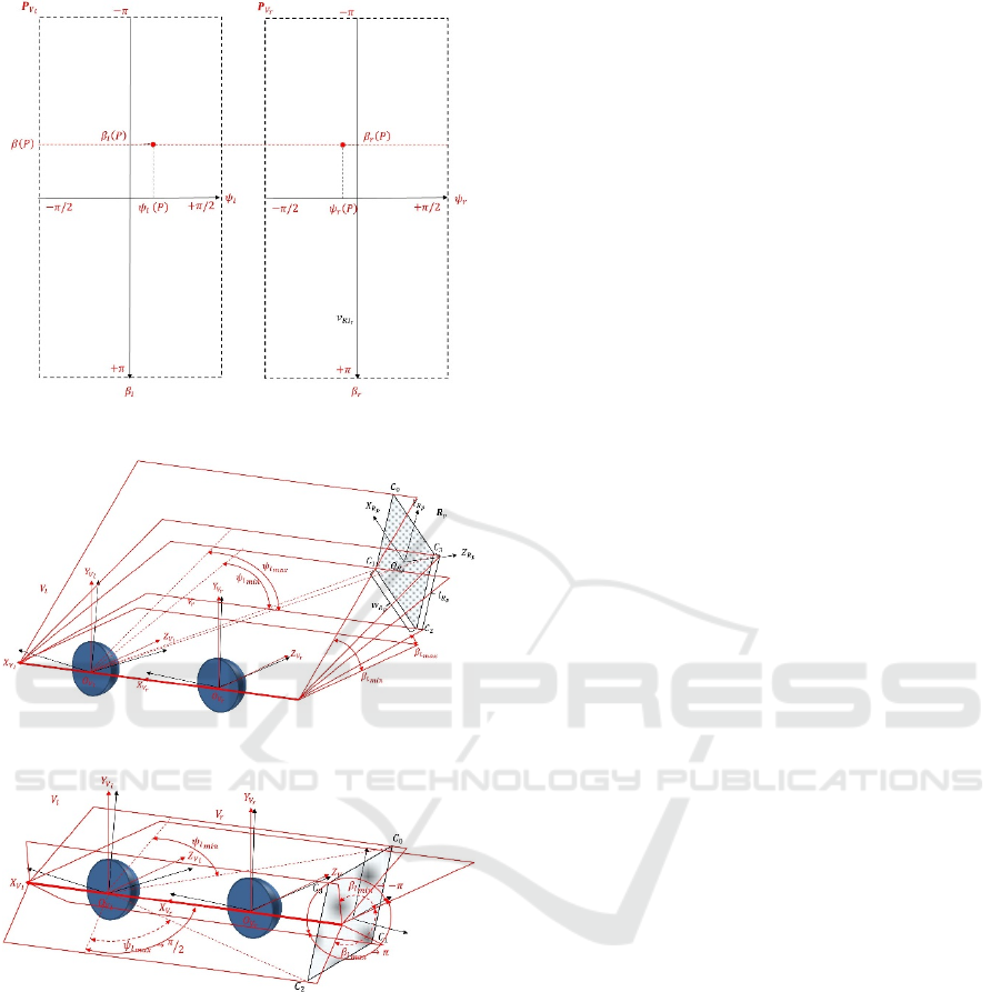
Figure 4: Projection planes.
Figure 5: Tilt and yaw angles including a reference plane.
Figure 6: Tilt and yaw angles including a reference plane
which crosses an extension of the stereo baseline.
coincides with
is the same direction as
to
.
is the direction of the cross product of
and
.
is the direction of the cross product of
and
.
is obtained by translating
to
.
Let us consider the light rays from a 3D point P to
the origins of the left and right virtual cameras,
and
. Their tilt angles
and
, which
are the angles of rotation around the X axes, are
equal. This is true for any 3D point. Then, any 3D
point is projected at the same vertical position on the
left and right projection planes,
and
, by
relating the vertical positions to the tilt angles. The
horizontal positions on the projection planes are
related to the yaw angles,
and
. Here
yaw angles are the angles of rotation around the
tilted Y axes. For convenience, the tilt angle is
defined in the counter clockwise direction from the
direction of the Z axes, while the yaw angle is
defined in the clockwise direction from the tilted Z
direction. The whole 3D space is projected into the
area for which the tilt angle ranges from π to –π
and the yaw angle ranges from 2
⁄
to 2
⁄
, as
shown in Figure 4.
3.2 Deciding the Rectifying Region
Only the rectangle-shaped portion of the projection
plane that contains a projection of the reference
plane is rectified rather than the whole projection
plane. The rectangle portion that has a tilt angle is
from
to
and a yaw angle is from
to
is decided in the left projection plane.
, for
0,1,2,3 , indicate the four corners of the
reference plane, as shown in Figure 5. Their
coordinates in the
frame are as follows.
2
⁄
,
2
⁄
,0
2
⁄
,
2
⁄
,0
2
⁄
,
2
⁄
,0
2
⁄
,
2
⁄
,0
(1)
The
are converted to the
frame through the
frame to yield
. The tilt and yaw angles in the
frame can be calculated as follows:
tan
sin
(2)
where
represents a X coordinate of
.
Finally, we find that
min
0,1,2,3
max
0,1,2,3
min
0,1,2,3
max
0,1,2,3
(3)
However, these values are updated when a reference
plane crosses an extension of the stereo baseline as
follows:
&
(4)
Reference Plane based Fisheye Stereo Epipolar Rectification
311
Further, if the X coordinate of the cross point in the
frame
is positive then
2
⁄
; otherwise,
2
⁄
, as shown in Figure 6.
3.3 Deciding Pixel Coordinate Frame
of Rectified Images
The pixel coordinate frame of the left rectified
image,
, is defined by equally quantizing the tilt
and yaw angles in the left projection plane. The
following two issues must be considered to choose
the quantizing resolution
.
I1.
affects the resolution of the 3D depth
measurement.
I2.
affects
, which is the Euclidean distance
on a reference plane corresponding to one pixel
of the rectified images.
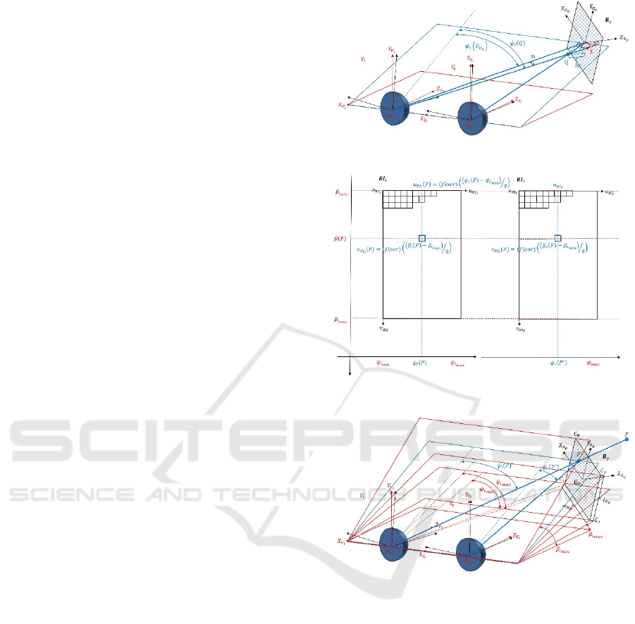
Figure 7 shows how to choose
based on the
desired depth resolution,
. A 3D point Q is set on
the light ray from
to
so that the Euclidean
distance between Q and the reference plane becomes
. The yaw angle of the light ray from Q to
is
, and one of the light rays from
to
is
. Then
is chosen according to:
(5)
The depth for one pixel disparity becomes about
around the center of the reference plane. For issue I2,
is calculated as the distance between
and S,
which is the intersection between the light ray from
Q to
and the reference plane. A larger
means
a small rectified image. If the calculated
is larger
than the threshold
, then point S is moved toward
on the reference plane so that the distance to
becomes
.
is recalculated by using S after
it has been moved.
By using the chosen value of
, the rectangle
region from
n to
and from
to
on the left projection plane is quantized, as shown in
Figure 8. The rectangle region on the right
projection plane is also quantized vertically using
.
The rectified image coordinates of a 3D point P,
,
and
,
, are obtained from the
following equations:
⁄
⁄
⁄
(6)
Because
,
and
,
is true for any 3D point P on the
rectified image.
Figure 7: Decision of
.
Figure 8: Pixel coordinate frames of rectified images.
Figure 9: Decision of a yaw angle for the pixel with the
coordinates
,
.
The horizontal quantization of the right
projection plane remains to be decided. It is
quantized non-linearly so that the disparity becomes
zero on the reference plane. The yaw angle in the
frame
for the pixel with the coordinates
,
is chosen as follows. First the tilt and yaw
angles of the light ray corresponding to the left pixel
,
, where
and
, are
obtained via the following equations:
0.5
0.5
(7)
Next, the point where the light ray and the reference
plane intersect, P’, is obtained as shown in Figure 9.
VISAPP 2017 - International Conference on Computer Vision Theory and Applications
312

Figure 10: Five poses of target planes.
Finally, the yaw angle in the frame
for the pixel
with the coordinates
,
is selected to be
′
. Using this approach, any 3D point on the
reference plane has the same coordinates in the left
and right rectified images. This results in the targets
having the same apparent shapes in the left and right
images when the targets are close to the reference
plane.
3.4 Conversion from Fisheye to
Rectified Image
For each pixel in the left rectified image, the
intensity is obtained as follows. The tilt and yaw
angle of the light ray corresponding to the pixel,
and
, are derived using Equation set 7. The unit
direction vector for the light ray,
, is obtained
according to:
sin
,cos
sin
,
,cos
cos
(8)
is then obtained by converting
to the
frame. The image coordinates in the left fisheye
image corresponding to the light ray are calculated
as real coordinates using the projection function
. Here, all intrinsic parameters of the left
fisheye camera were calibrated in advance. From the
intensities of the four neighboring pixels in the left
fisheye image, the intensity value of the pixel in the
left rectified image was calculated via linear
interpolation.
For each pixel in the right rectified image, the
intensity was obtained in the almost same way as for
one in the left rectified image. First, the
for the
same coordinate in the left rectified image was
obtained. Then,
was converted to
and
was obtained as a light ray from the intersection
between
and the reference plane toward
.
The image coordinates in the right fisheye image
corresponding to the light ray are calculated by the
function
. From the intensities of the four
neighboring pixels in the right fisheye image, the
intensity value of the pixel in the right rectified
image was calculated via linear interpolation.
4 EXPERIMENTS
The motivation for proposing a new rectification
method is to enable 3D distance measurements for
targets in close proximity at wide angles, so as to
include the line extended from the stereo baseline.
Additionally, it should be possible to measure the
distances using a simple matching method even
when the texture of the targets is poor. Actual
fisheye stereo image pairs were rectified using the
proposed method, and 3D distance measurements
were performed using simple region-based matching
on the rectified images. For the comparison, another
rectification method was used on the same images
and the 3D distances were measured from the
rectified images using the same matching method.
4.1 Experimental Setup
The fisheye stereo that was used for the experiments
was mounted on the chest of a humanoid robot; the
baseline length was about 150 mm and the directions
of optical axes were set to point forward, as shown
in Figure 1. The field of view of the fisheye lenses
were each 214° with an almost spherical projection.
The cameras captured the whole viewing field with
1536 1536 pixel images.
The targets were two kinds of flat veneer
surfaces that were 300 mm 300 mm in size. One
surface was given a rich texture by placing a section
of newspaper on it, while the other was left blank
and was thus poorly textured. The targets were fixed
at five poses as shown in Figure 10. The poses were
chosen such that they were in poses that the
humanoid robot would be able to touch with its right
hand to stabilize itself. The positions and
orientations of the five poses were as follows.
Pose 0. (75, 0, 200), (0, 0, 0),
Pose 1. (−200, 0, 100), (0, −90, 0),
Pose 2. (−200, 0, 300), (0, −90, 0),
Pose 3. (−200, 200, 100), (0, −90, 0),
Pose 4. (75, 250, 100), (−90, 0, 0).
The positions and orientations were based on the
frame
, which is the same as for the reference
plane. The position coordinates are given in
millimeters, while the orientations are given in
degrees. The orientation is represented by YXZ
Reference Plane based Fisheye Stereo Epipolar Rectification
313
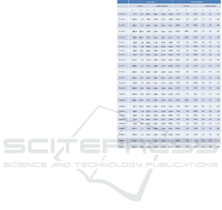
Euler angles. Because it was difficult to fix the
targets at the intended poses, the actual poses were
slightly different and the actual poses that were
measured using the method described in Section 4.4
are shown in Table 1. For convenience, a name is
given to each pair of stereo images, e.g., 0-rich-0,
where the first number represents a pose between 0
and 4, the second indicates the surface type (rich or
poor, i.e., richly or poorly textured), and the third
number represents the orientation (0–4). The
orientation numbers have the following significance:
0: base orientation
1: rotate 0 about 10° around Y axis
2: rotate 0 about −10° around Y axis
3: rotate 0 about 10° around X axis
4: rotate 0 about −10° around X axis
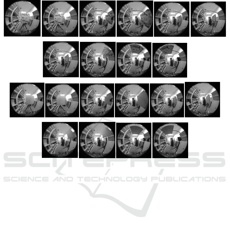
The rich and poor input image pairs at the five poses
with the base orientations are shown in Figure 11.
The images were captured for orientation 0 for every
position. Only for positons 0 and 1 were the images
captured for orientations 1 to 4.
4.2 Rectification of Fisheye Images
In the proposed rectification method a reference
plane is set to decide which portion of the fisheye
images should be rectified. The size of rectified
images is determined by setting a desired depth
resolution,
, and a threshold for
,
. The
process introduced in Section 3.4 generates rectified
images based on the reference plane. Here three
typical examples are presented.
Example 1. Dimensions of a reference plane:
250 ,
250 . Pose:
75,0,200
,
0,0,0
. Further,
is −51.2,
=
49.6,
= −17.6, and
= 52.3.
and
are set to 10 and 2, respectively. Now
is 2.11.
Because this is larger than
,
is updated to 1.3
so that
is equal to
. Then,
is 0.684 and the
size of the rectified images is 124 172. Generated
rectified images from 0-rich-0 are shown in Figure
12(a).
Example 2. Dimensions of a reference plane:
250 ,
250 . Pose:
200,0,100
,
0,90,0
. Further,
is ,
= ,
= 50.9, and
= 73.1.
and
are set to 10 and 2, respectively. Now
is
2.11. Because this is larger than
,
is updated to
9.49 so that
is equal to
. Then,
is 0.297 and
the size of the rectified images is 152 1232.
Generated rectified images from 1-rich-0 are shown
in Figure 12(b).
Table 1: Target poses and reference plane poses.
Example 3. Dimensions of a reference plane:
250 ,
250 . Pose:
200,300,100
,
0,90,0
. Further,
is -95.7,
= -20.7,
= 38.9, and
= 75.4.
and
are set to 10 and 2,
respectively. Now
is 4.83. Because this is larger
than
,
is updated to 4.21 so that
is equal to
. Then,
is 0.228 and the size of the rectified
images is 184 352. Generated rectified images
from 3-rich-0 are shown in Figure 12(c).
Because the reference planes are set close to the
actual targets in all three examples, the apparent
shape of the targets on the rectified images are quite
similar.
For comparison, another rectification method
was implemented by referring to Abraham. This
method rectifies fisheye images of the whole
projection plane with equal quantization amounts
for both the vertical and horizontal directions. Thus,
the typical difference in the implementation of this
method and the proposed method is the relation
between the yaw angles and the horizontal pixel
coordinates on the right rectified image according to
⁄
(9)
VISAPP 2017 - International Conference on Computer Vision Theory and Applications
314
0-rich-0 1-rich-0 2-rich-0
3-rich-0 4-rich-0
0-poor-0 1-poor-0 2-poor-0
3-poor-0 4-poor-0
Figure 11: Input fisheye images.
For the remainder of this paper, this rectification is
referred to as the Abraham method. As for the above
Examples 1, 2, and 3, the Abraham method was
applied to 0-rich-0, 1-rich-0, and 3-rich-0 and the
generated rectified images are shown in Figure 13.
The obtained quantization amount
was the same
as with the proposed method with a reference plane
and the two parameters
and
. The sizes of the
rectified images are 396 768, 628 1232, and 812
1604.
4.3 3D Distance Measurements
In the rectified images, corresponding pairs were
identified with a region-based method using NSSD
(Davison, 1998) as the measure of dissimilarity. The
necessary parameters are listed here.
patch_size: the size of the local region where the
NSSD is calculated. Here it was 21 pixel.
corr_th: threshold of the dissimilarity for
acceptance as a matching pair. Here it was 1.5.
corr_diff_th: threshold of the saliency for
acceptance as a matching pair. Here it was 0.5.
max_d: search was performed within this
distance from the reference plane. Here it was 200
mm.
For each pixel in the left rectified image, stereo
matching is carried out as follows if the
corresponding light ray crosses with the reference
plane. Between pixel
,
in the left rectified
image and the pixels in the right rectified images
that have the same and lie between
_
⁄
and
_
⁄
, the
NSSD was calculated for the local region with a
size: patch_size patch_size. If the minimum value
of the NSSDs is lower than corr_th and the
differences between the NSSDs of the horizontal
neighbors are larger than corr_diff_th, the pixel is a
matching candidate. Using the same process, the
matching candidate in the left rectified image is
determined via a reverse searched from the matching
candidates in the right rectified image. If the found
pixel is
,
, the pair is as a matching pair.
For the images rectified by the Abraham method,
the same procedure with the same parameters was
applied with only one exception: the search area was
defined as lying between
_
⁄
Reference Plane based Fisheye Stereo Epipolar Rectification
315
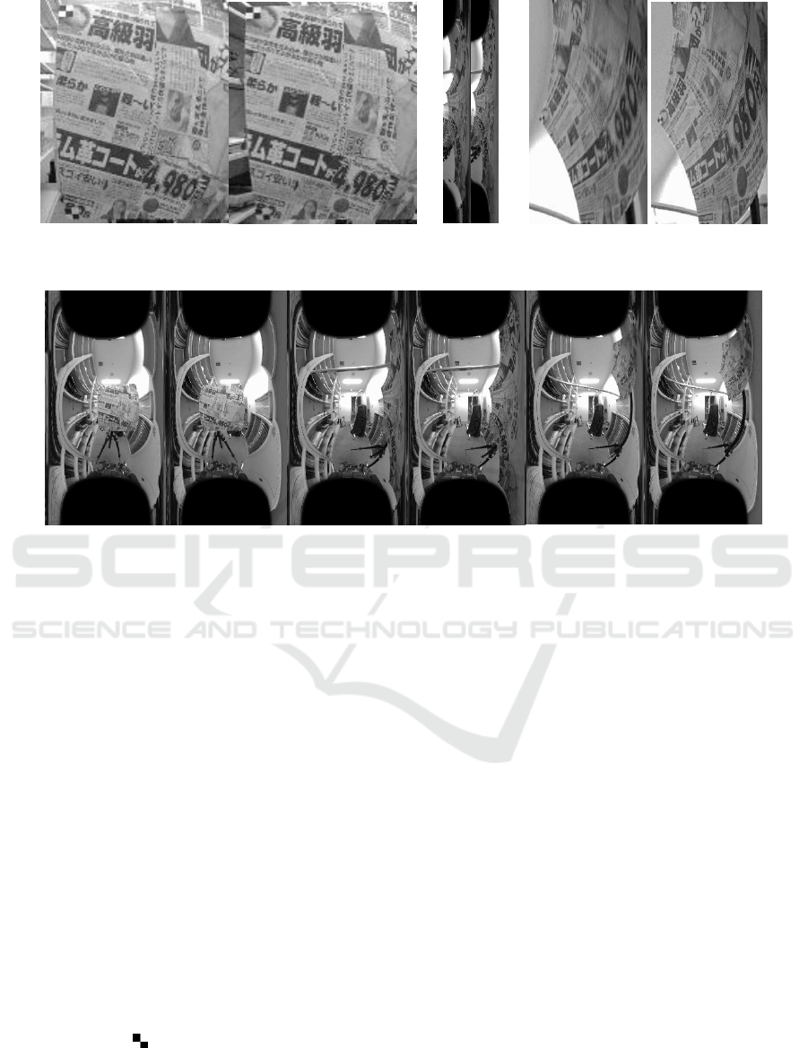
(a) (b) (c)
Figure 12: Rectified images by the proposed method.
(a) (b) (c)
Figure 13: Rectified images by Abraham method.
and
_
⁄
by using d, which is
the disparity on the reference plane.
For the matching pairs, the 3D location was
calculated as the crossing point of the corresponding
left and right rays.
4.4 Evaluation Criteria
The total number, TN, is defined as the number of
the pixels for which the stereo matching was carried
out. The matching number, MN, is defined as the
number of matching pairs. The correct number, CN,
is defined as the number of matching pairs from
which a 3D location is calculated and for which the
distance between it and the actual target plane was
less than the threshold,
. The following
evaluation criteria were used:
MN/TN,
CN/MN.
The actual pose of the target plane was obtained
from the left and right fisheye images by detecting
the cross marks, , that were placed at the four
corners of the target. The threshold
was 10 mm.
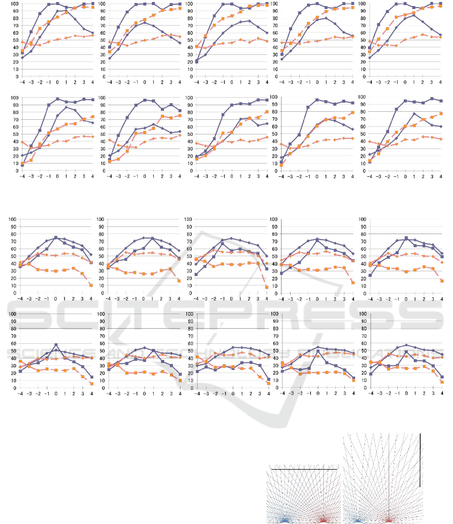
4.5 Experimental Results
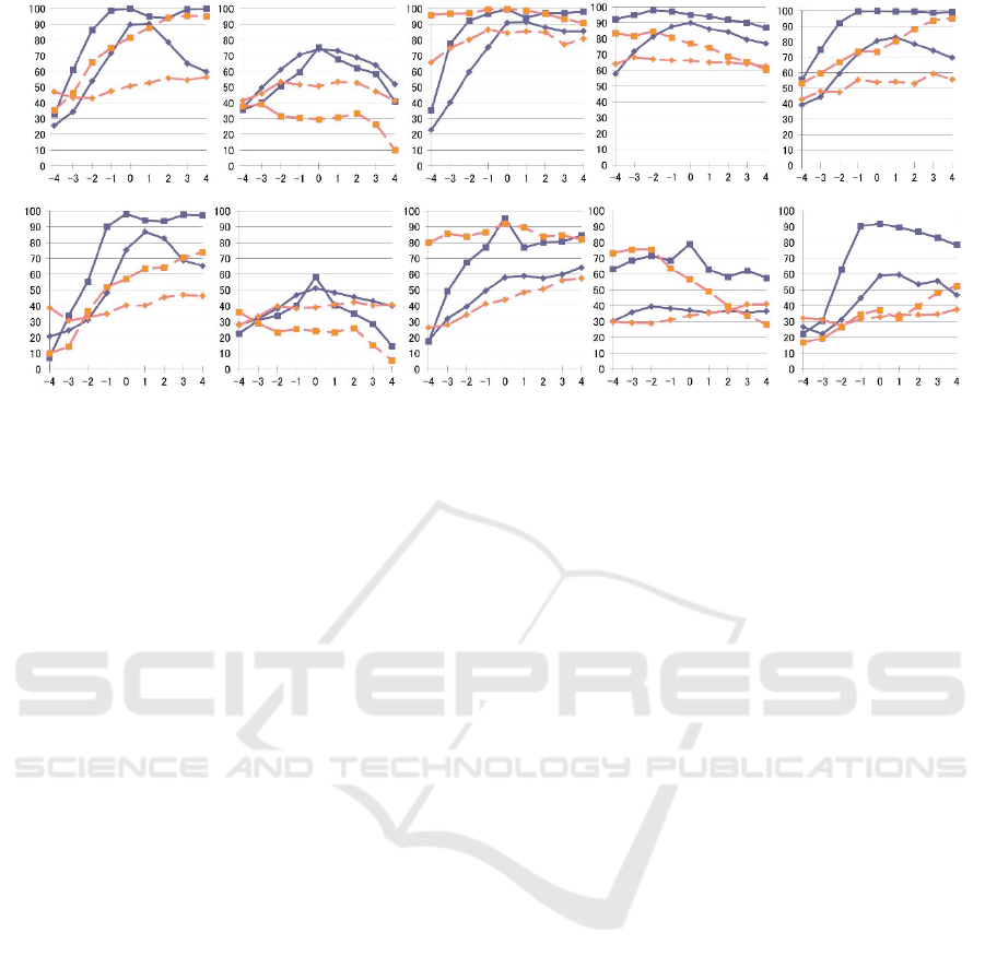
Figure 14 shows the results obtained from the
fisheye image pairs at the five poses with the base
orientation. Figure 15 shows the results obtained
from the fisheye image pairs at pose 0 with the five
orientations. Figure 16 shows the results obtained
from the fisheye image pairs at pose 1 with the five
orientations. Blue represents the results obtained by
using the proposed rectification method and orange
represents the results obtained using the Abraham
method. The + symbols indicate the values of
MN/TN 100, while the ■ symbols represent the
values of CN/MN 100. For each input image pair,
the 3D distances were measured nine times for
various reference plane positions. The numbers from
−4 to 4 on the horizontal axis, k, correspond to the
positions of the reference planes, where 0 is the base
position, which is the closest to the actual target
plane. –k means that the reference plane is moved
toward the cameras along the normal direction of the
reference plane at (k 25) mm from the base
position. +k means that the reference plane is moved
away from the cameras along the normal direction of
the reference plane at (k 25) mm from the base
VISAPP 2017 - International Conference on Computer Vision Theory and Applications
316
0-rich-0 1-rich-0 2-rich-0 3-rich-0 4-rich-0
0-poor-0 1-poor-0 2-poor-0 3-poor-0 4-poor-0
Figure 14: Results obtained from the fisheye image pairs at the five poses with the base orientation.
position. To obtain the results for Figures 15 and 16,
the same reference plane orientation was used
independent of the actual orientation of the target.
Table 1 shows the actual pose of targets and the pose
of reference planes at the base position.
Prior to conducting the experiments, the
following five phenomena were predicted to occur.
E1. With the proposed method, the results should
worsen as |k| increases.
E2. With the Abraham method, the results should
be almost constant independent of |k|.
E3. The results of the proposed method should be
better than ones of the Abraham method when
|k| is small.
E4. The results for poor textures should be worse
than for rich textures; however, for positions at
which |k| is small, reasonable results should be
obtained using the proposed method.
E5. The effect of the orientation difference between
the target and reference planes should be much
smaller than that caused by the positional
difference between the target and reference
planes.
Based on the results shown in Figure 14, the
expectations E1 to E4 are supported as follows. E1
was true for pose 0. For poses 0, 2, and 4 the results
for larger k did not worsen and for pose 3 the results
did not change significantly regardless of the values
of k. E2 was not true; the results monotonically
increased or decreased along with the positional
changes. This seems to be caused by the changes in
the amount of quantization. E3 held true except for
pose 2. Figure 17 depicts the changes in Euclidean
distance on the reference plane corresponding to one
pixel when the yaw angles are equally quantized on
the left and right rectified images, as in the Abraham
method. Figure 17(a) is for pose 0 and (b) for pose 2.
As seen in Figure 17(a), the Euclidean distances on
the reference plane corresponding to one pixel were
quite different between the left and right images; this
causes the difference in the apparent shape in the
rectified images even when the target resides on the
reference plane. Conversely, for pose 2, the
Euclidean distances on the reference plane
corresponding to one pixel were almost the same
between the left and right images, which causes
apparent shape in the left and right rectified images
to be similar even when the target is not on the
reference plane. This causes the results for pose 2 at
any position using the Abraham method to be almost
the same as those obtained at position 0 using the
proposed method. As expected according to E4, the
results for the poor texture were worse than those for
the rich texture for both the Abraham and the
proposed method. For pose 1, which is the most
challenging configuration for a stereo measurement,
the CN/MN was less than 25% for the Abraham
method. Conversely, using the proposed method, the
CN/MN was greater than 40% for |k| < 2. Figure 18
shows the results of the 3D distance measurements
for pose 1 of poor texture. The upper two rows are
for the proposed method and the lower two rows are
for the Abraham method. White solid rectangles
indicate the cameras. The white solid lines show the
viewing directions of the cameras. Further, white
dots represent the measured results. Additionally,
the red squares show the reference planes.
Estimating whether a real plane does or does not
exist in the measurement area and estimating the
pose of the plane if it does exist appears to be
difficult to achieve from the point clouds obtained
by the Abraham method. However, from the point
Reference Plane based Fisheye Stereo Epipolar Rectification
317
0-rich-0 0-rich-1 0-rich-2 0-rich-3 0-rich-4
0-poor-0 0-poor-1 0-poor-2 0-poor-3 0-poor-4
Figure 15: Results obtained from the fisheye image pairs at pose 0 with the five orientations.
1-rich-0 1-rich-1 1-rich-2 1-rich-3 1-rich-4
1-poor-0 1-poor-1 1-poor-2 1-poor-3 1-poor-4
Figure 16: Results obtained from the fisheye image pairs at pose 1 with the five orientations.
clouds obtained by the proposed method for |k| < 2,
making such an estimation appears to be possible
with only simple post processing.
Based on the results shown in Figures 15 and 16,
E5 is true.
(a) (b)
Figure 17: Changes in Euclidean distance on the reference
plane corresponding to one pixel when the yaw angles are
equally quantized on the left and right rectified images.
VISAPP 2017 - International Conference on Computer Vision Theory and Applications
318
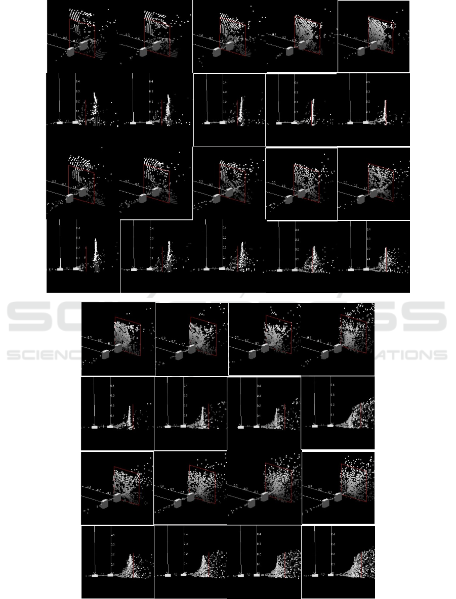
k=-4 k=-3 k=-2 k=-1 k=0
k=1 k=2 k=3 k=4
Figure 18: Results of the 3D distance measurements for pose 1 of poor texture.
Reference Plane based Fisheye Stereo Epipolar Rectification
319

5 CONCLUSIONS
We proposed a new epipolar rectification method for
fisheye images. It rectifies a portion of the fisheye
images so that the apparent shape on the left and
right rectified images becomes similar if a target is
close to a reference plane. By using the proposed
method and setting the reference plane appropriately,
the 3D distances of a target plane can be measured
using a simple region-based matching method, even
if the target plane lies within reach of the robot to
which the cameras are mounted and even if it lies in
the direction of the extension of the stereo baseline.
The superiority of the proposed method was
experimentally compared with another method to
validate it.
We are now developing a method to judge the
existence of a plane and estimate the pose of the
plane should it exist based on the proposed method;
this method will be applied for the motion planning
of a humanoid robot when it needs to contact any
part of its upper body with the environment to retain
its balance.
REFERENCES
Sentis, L., 2010. Compliant control of whole-body multi-
contact behaviors in humanoid robots. Motion
Planning for Humanoid Robots, Springer: 29-66.
Escande, A., A. Kheddar, et al., 2013. Planning contact
points for humanoid robots. Robotics and Autonomous
Systems 61(5): 428-442.
Henze, B., M. A. Roa, et al., 2016. Passivity-based whole-
body balancing for torque-controlled humanoid robots
in multi-contact scenarios. The International Journal of
Robotics Research: 0278364916653815.
Brossette, S., J. Vaillant, et al., 2013. Point-cloud multi-
contact planning for humanoids: Preliminary results.
6th IEEE Conference on Robotics, Automation and
Mechatronics (RAM), IEEE.
Khatib, O. and S.-Y. Chung, 2014. SupraPeds: Humanoid
contact-supported locomotion for 3D unstructured
environments. IEEE International Conference on
Robotics and Automation (ICRA), IEEE.
Schmid, C. and A. Zisserman, 1997. Automatic line
matching across views. Computer Vision and Pattern
Recognition..
Baumberg, A., 2000. Reliable feature matching across
widely separated views. Computer Vision and Pattern
Recognition.
Matas, J., O. Chum, et al., 2004. Robust wide-baseline
stereo from maximally stable extremal regions. Image
and vision computing 22(10): 761-767.
Bay, H., V. Ferrari, et al., 2005. Wide-baseline stereo
matching with line segments. Computer Vision and
Pattern Recognition.
Scharstein, D. and R. Szeliski, 2002. A taxonomy and
evaluation of dense two-frame stereo correspondence
algorithms. International Journal of Computer Vision
47(1-3): 7-42.
Hartley, R. and A. Zisserman, 2003. Multiple view
geometry in computer vision, Cambridge university
press.
Ayache, N. and C. Hansen, 1988. Rectification of images
for binocular and trinocular stereovision. 9th
International Conference on Pattern Recognition.
Courtney, P., N. A. Thacker, et al., 1992. A Hardware
Architecture for Image Rectification and Ground Plane
Obstacle Avoidance. Proc. 11th ICPR 1992.
Loop, C. and Z. Zhang, 1999. Computing rectifying
homographies for stereo vision. Computer Vision and
Pattern Recognition.
Hartley, R. I., 1999. Theory and Practice of Projective
Rectification. Int. J. Comput. Vision 35(2): 115-127.
Hirschmuller, H. and D. Scharstein, 2009. Evaluation of
stereo matching costs on images with radiometric
differences. IEEE Transactions on Pattern Analysis
and Machine Intelligence 31(9): 1582-1599.
Zabih, R. and J. Woodfill, 1994. Non-parametric local
transforms for computing visual correspondence.
European conference on computer vision, Springer.
Geiger, A., M. Roser, et al., 2010. Efficient large-scale
stereo matching. Asian conference on computer vision,
Springer.
Hirschmuller, H., 2008. Stereo processing by semiglobal
matching and mutual information. IEEE Transactions
on Pattern Analysis and Machine Intelligence 30(2):
328-341.
Devernay, F. and O. D. Faugeras, 1994. Computing
differential properties of 3-D shapes from stereoscopic
images without 3-D models. Computer Vision and
Pattern Recognition.
Tola, E., V. Lepetit, et al., 2010. Daisy: An efficient dense
descriptor applied to wide-baseline stereo. Pattern
Analysis and Machine Intelligence, IEEE Transactions
on 32(5): 815-830.
Kita, N., 2011. Direct floor height measurement for biped
walking robot by fisheye stereo. 11th IEEE-RAS
International Conference on Humanoid Robots.
Pollefeys, M., R. Koch, et al., 1999. A simple and efficient
rectification method for general motion. The
Proceedings of the Seventh IEEE International
Conference on Computer Vision.
Abraham, S. and W. Förstner, 2005. Fish-eye-stereo
calibration and epipolar rectification. ISPRS Journal of
Photogrammetry and Remote Sensing 59(5): 278-288.
Davison, A., 1998. Mobile Robot Navigation Using
Active Vision. D. Phil Thesis, University of Oxford.
VISAPP 2017 - International Conference on Computer Vision Theory and Applications
320
