
Saliency Sandbox
Bottom-up Saliency Framework
David Geisler, Wolfgang Fuhl, Thiago Santini and Enkelejda Kasneci
Perception Engineering, University of T
¨
ubingen, T
¨
ubingen, Germany
{david.geisler, wolfgang.fuhl, thiago.santini, enkelejda.kasneci}@uni-tuebingen.de
Keywords:
Saliency Sandbox, Feature Maps, Attention Maps, Saliency Maps, Bottom Up.
Abstract:
Saliency maps are used to predict the visual stimulus raised from a certain region in a scene. Most approaches
to calculate the saliency in a scene can be divided into three consecutive steps: extraction of feature maps,
calculation of activation maps, and the combination of activation maps. In the past two decades, several new
saliency estimation approaches have emerged. However, most of these approaches are not freely available as
source code, thus requiring researchers and application developers to reimplement them. Moreover, others are
freely available but use different platforms for their implementation. As a result, employing, evaluating, and
combining existing approaches is time consuming, costly, and even error-prone (e.g., when reimplementation
is required). In this paper, we introduce the Saliency Sandbox, a framework for the fast implementation and
prototyping of saliency maps, which employs a flexible architecture that allows designing new saliency maps
by combining existing and new approaches such as Itti & Koch, GBVS, Boolean Maps and many more. The
Saliency Sandbox comes with a large set of implemented feature extractors as well as some of the most popular
activation approaches. The framework core is written in C++; nonetheless, interfaces for Matlab and Simulink
allow for fast prototyping and integration of already existing implementations. Our source code is available
at: www.ti.uni-tuebingen.de/perception.
1 INTRODUCTION
Human visual perception is directly linked to eye
movements. During fixations, visual information is
extracted and processed, whereas saccades are per-
formed to change the focused area (Tafaj et al., 2012).
Selectivity of these areas is known as visual attention
and depends on the visual stimuli as well as on the
intention of the beholder (Patrone et al., 2016). One
of the earliest models of human visual attention was
proposed by (Treisman and Gelade, 1980), who in-
vestigated the effect of different visual stimuli on vi-
sual attention and identified a set of attractive visual
features. Conversely, the visual stimulus can be deter-
mined by extracting intrinsic scene features (so-called
bottom-up) followed by a model of the visual input
processing in the eye. In contrast, top-down models
predict the visual attention accrued from high-level
processing of the scene and context.
In bottom-up models, an area of the scene is con-
sidered salient if it stands out from its local neigh-
borhood (Patrone et al., 2016). Activation maps re-
veal high responses on salient areas at feature level,
which correspond to a high neural activation of the
visual processing in a biological manner. For in-
stance, the bottom-up computational approach pro-
posed by (Itti and Koch, 2000) models the recep-
tive field of an individual sensory neuron, whereas
GBVS uses graphs to model the retinotopically or-
ganized network in the visual cortex (Harel et al.,
2006a). Other methods determine the saliency of an
area based on frequency analysis (e.g., the Frequency
Tuned Saliency approach (Achanta et al., 2009), or
methods provided by the Spectral Saliency Toolbox
(Schauerte and Stiefelhagen, 2012; Hou and Zhang,
2007)). Combining several activation maps leads to
a saliency map, which states the saliency of differ-
ent visual features and sums them to a predicted vi-
sual stimulus (Von Goethe, 1840; Itti and Koch, 2000;
Harel et al., 2006a; Achanta et al., 2009; Zhang and
Sclaroff, 2013). There are already several imple-
mentations providing saliency maps algorithms. Be-
sides the aforementioned Spectral Saliency Toolbox,
the Saliency Toolbox (Walther and Koch, 2006) im-
plements the Itti & Koch method (Itti and Koch, 2000;
Itti, 2004). Furthermore, an implementation of the
GBVS algorithm together with an Itti & Koch saliency
map is provided by (Harel et al., 2006a; Harel et al.,
2006b). The above approaches were implemented in
Matlab and were designed for rapid application of
Geisler D., Fuhl W., Santini T. and Kasneci E.
Saliency Sandbox - Bottom-up Saliency Framework.
DOI: 10.5220/0006272306570664
In Proceedings of the 12th International Joint Conference on Computer Vision, Imaging and Computer Graphics Theory and Applications (VISIGRAPP 2017), pages 657-664
ISBN: 978-989-758-225-7
Copyright
c
2017 by SCITEPRESS – Science and Technology Publications, Lda. All rights reserved
657

the predefined saliency maps. Merely the Toolbox
by (Harel et al., 2006b) allows a simple extension of
the already defined feature maps. None of these ap-
proaches was developed for designing new algorithms
by combining already existing feature and activation
maps or to extend already existing approaches with
your own. Even if some toolboxes use precompiled
and speed optimized Mex-functions, the Matlab en-
vironment generates an overhead in calculation time.
Using a native C++ environment to calculate saliency
maps can produce a significant speed-up
1
.
In this paper, we introduce the Saliency Sandbox,
a framework for developing bottom-up saliency maps.
Our main goal is to provide a flexible back-end that
can be used to develop and prototype new saliency
estimation approaches in a quick and standardized
manner. By providing S-Functions for Simulink, the
Saliency Sandbox allows the use in a real-time sig-
nal processing environment, such as in the automo-
tive context, where the question whether objects on
the scene have been perceived by the driver might be
solved by combining eye-tracking data with saliency
information of the scene (Kasneci et al., 2015).
The key advantages of Saliency Sandbox are:
Research Speed-up: The code is freely available,
i.e., users can easily integrate their own algo-
rithms or employ already provided feature extrac-
tors and activation models to combine them and
create new saliency maps. Interfaces for Matlab
facilitate the integration of existing toolboxes.
Processing Time: Written in C/C++, our framework
accesses the full computational power of the ma-
chine. The GPU is accessible via Cuda and
OpenCV, providing a significant speed-up through
parallelization. In addition, Simulink S-Functions
allow the use in a real-time signal processing en-
vironment such as automotive or robotics.
Streaming: Calculate saliency maps on videos as
well as on individual frames. We already pro-
vide several utilities to improve your results using
sequential data, such as optical flow for tracking
saliency, or background subtraction as a new kind
of feature map.
State-of-the-art Saliency Maps: The Saliency
Sandbox provides a large selection of feature
extractors together with the most famous activa-
tion models such as Itti & Koch (Itti and Koch,
2000), GBVS (Harel et al., 2006a), Frequency
Tuned Saliency (Achanta et al., 2009), Spectral
1
We reached a speed-up factor of ≈ 2.2 calculating a GBVS
activation compared to the toolbox introduced in (Harel
et al., 2006b).
whitening (Hou and Zhang, 2007), and Boolean
Maps (Zhang and Sclaroff, 2013).
The following sections describe the architecture of the
Saliency Sandbox, the delivered feature extractors and
activation models, as well as a sample usage.
2 ARCHITECTURE
The Saliency Sandbox considers the process from raw
input image to Saliency map output as a tree with pro-
cessing steps as node structures that provide an in-
put and output. The root node usually combines sev-
eral activation maps. Each activation map leads to a
branch connected with the root node. Usually, an acti-
vation map depends on a feature extractor, which can
lead to further branches and nodes. Figure 1 shows
an example of how the Saliency Sandbox implements
the Itti & Koch approach as a processing tree. Each
node is represented by a uniform interface with an in-
put and output buffer. This allows an arbitrary com-
bination of features and activations. Thus, it is also
possible to experiment in the hierarchy – e.g., by us-
ing a saliency map as activation. The tree architec-
ture comes with the advantage that each branch can
be calculated independently, which allows a speed-
up through parallelization, but may cause a redundant
calculation of some features. The Saliency Sandbox
implements a producer-consumer model to limit the
number of threads to an optimal amount regarding the
CPU capabilities.
Each node implements the abstract base class Algo-
rithm (see Figure 2). This abstract class provides ba-
sic functionalities such as input and output buffers, in-
terfaces for Matlab and Simulink, and properties for
parameterization. Algorithms processing images and
videos can implement the specialization ImageAlgo-
rithm, which already provides functions to convert
RGB images to the appropriate input type and size,
or utilities for loading and processing videos. The ab-
stract methods reset and calc are called by the Algo-
rithm base class and implement the actual algorithm.
The method reset sets the algorithm to a default state,
whereas calc calculates the output based on the input
and parameters.
Besides the interfaces to Matlab and Simulink, al-
gorithms from the Saliency Sandbox can also be inte-
grated into existing projects as a library or executed as
a standalone tool. For the latter, the base class Algo-
rithm and the ImageAlgorithm class provide methods
for, e.g., parsing call parameters as algorithm prop-
erties or loading inputs such as images, videos, or
masks to limit the calculation space.
Using the provided cmake-based build system,
VISAPP 2017 - International Conference on Computer Vision Theory and Applications
658
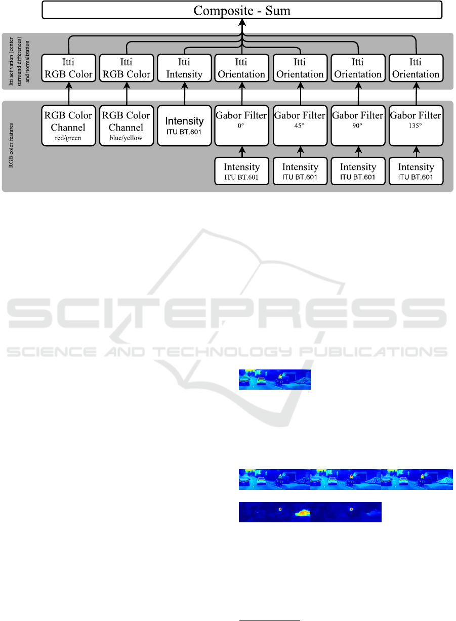
Figure 1: Implementation of the (Itti and Koch, 2000) model in the Saliency Sandbox. The activation is calculated by center
surround differences using pyramids of seven scales and normalization by iteratively DoG filtering, followed by a rectification.
All features are extracted from the RGB colorspace. The RGB Color Channel feature extracts a certain channel from the RGB
colorspace or in this case the pseudo channel as differences of red and green respectively blue and yellow. The intensity is
calculated in the standard ITU BT.601 (ITU, 2011). The orientation features are extracted by Gabor filters with different
rotations (0
◦
, 45
◦
, 90
◦
, 135
◦
). The composition of the activations maps is realized by a weighted sum (Itti and Koch, 2000).
the created binaries contain all the dependencies to
OpenCV 2.4 and Boost, which enables portability
between different systems. Thus, new libraries and
programs can be created without modification of the
build scripts.
3 ALGORITHMS
The Saliency Sandbox comes with a large set of Fea-
ture and activation maps. Most of them make exten-
sive use of the OpenCV 2.4 library for image process-
ing and GPU handling. Figure 4 provides an overview
of the currently implemented feature and activation
maps. In the following three sections, we will give
a short introduction of each implemented algorithm
followed by an example output. A short driving scene
recorded with an action cam placed behind the wind-
shield was used as input. Driving scenes are a hard
challenge for motion based features as the ego mo-
tion causes a ubiquitous change in the image. Figure 3
shows the corresponding input image at the time these
outputs shown here were created. We highly recom-
mend viewing these examples in color/digital form.
3.1 Features
We distinguish between three types of features: color
features extract channels or their contrast in a cer-
tain color space (RGB, LMS, DKL, LAB), frequency
features are represented by Gabor filters, and motion
features are used to examine sequences of images by
their optical flow, background subtraction, or flicker.
Intensity: The intensity is calculated according to
the ITU BT.601 standard, i.e., as a weighted sum of
the RGB channels (ITU, 2011):
I = 0.299 ×R +0.587 ×G + 0.114 × B (1)
I
RGB: Features from the RGB color space can be the
RGB channels themselves. Inspired by the structure
of the retinal ganglion cells, Itti & Koch extracted the
difference of yellow
2
and blue (Y − B) as well as red
and green (R − G) as features (Itti and Koch, 2000).
R
G
B
Y − B
R − G
Lab: The Lab color space describes the luminance
in the channel L, as well as the opponent colors
red-green (channel a) and yellow-blue (channel b).
It is a transformation to the CIE-XYZ color space to
achieve an equidistance in the change of color values
and the actual color perception of humans. Both,
Frequency Tuned Saliency maps and Boolean Maps,
2
Y = R + G
Saliency Sandbox - Bottom-up Saliency Framework
659
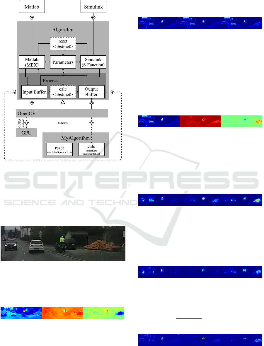
Figure 2: The abstract Algorithm base class provides inter-
faces for Matlab and Simulink and implements the buffers
for input and output. Furthermore, this class provides
a property handling for parameterizable algorithms. The
buffers are described using OpenCV data types. The inte-
gration of OpenCV allows access to a wide range of exist-
ing image processing functions and easy access to the GPU.
New algorithms just have to implement the abstract func-
tions reset and calc to provide new functionalities to the
Saliency Sandbox.
Figure 3: Input image showing a driving scene. The mo-
torcyclist with the yellow warning vest should have a high
saliency as expected.
use the LAB color space as features (Achanta et al.,
2009; Zhang and Sclaroff, 2013).
L
a
b
LMS: The LMS color space describes the response
of the three cones of the human eye. The L-channel
represents the long wavelength receptor, which is
responsible mainly for the red light perception. M
represents the medium wavelength receptor, which
covers the light between blue and orange. The last
channel S represents the short wavelength receptor
and covers blue light.
L M
S
DKL: The Derrington-Krauskopf-Lennie color
space is a Cartesian representation of the LMS color
space. The DKL color space respects the linear
combination model of signals from the cones to
perceive colors and luminance. Along the I + M
axis, only the perceived luminance changes, without
affecting the chromaticity. The axis I − M varies
the chromaticity without changing the excitation
of the blue sensitive cone. Along S − (I + M) the
chromaticity varies without impact to the red-green
sensitivity (Derrington et al., 1984).
L + M
L − M
S − (L + M)
Contrast: The contrast feature σ
f
(I) is calculated as
a local standard deviation. For this, the local mean
ˆ
E(I) is estimated by a Gaussian filter. The local stan-
dard deviation is calculated as
σ
f
(I) =
q
ˆ
E((I −
ˆ
E(I))
2
). (2)
The variance σ
2
of the Gaussian filter determines the
locality of the standard deviation.
σ
f
(L + M) σ
f
(L − M) σ
f
(S − (L + M))
Orientation: Many saliency maps extract orienta-
tional features, since Treisman and Glades discovered
that the orientation of objects is related to the visual
stimuli (Treisman and Gelade, 1980). Itti & Koch
as well as J. Harel (GBVS) use Garbor filters G
f
(I)
with different rotations to encode local orientation
contrast (Itti and Koch, 2000; Harel et al., 2006a).
G
f
(L + M) G
f
(L − M) G
f
(S − (L + M))
Flicker: The method by Harel et al. (Harel et al.,
2006b) provides Flicker as an optional feature
w.r.t. motion in sequential images. The Flicker
feature is defined as the absolute difference of
two subsequent images (Harel et al., 2006b):
F
f
(I
i
, I
i−1
) =
p
(I
i
− I
i−1
)
2
F
f
(L
i
+ M
i
, L
i−1
+ M
i−1
) F
f
(L
i
− M
i
, L
i−1
− M
i−1
)
F
f
(S
i
− (L
i
+ M
i
), S
i−1
−
(L
i−1
+ M
i−1
))
Background: In accordance with the Flicker feature,
the Saliency Sandbox provides various methods for
VISAPP 2017 - International Conference on Computer Vision Theory and Applications
660
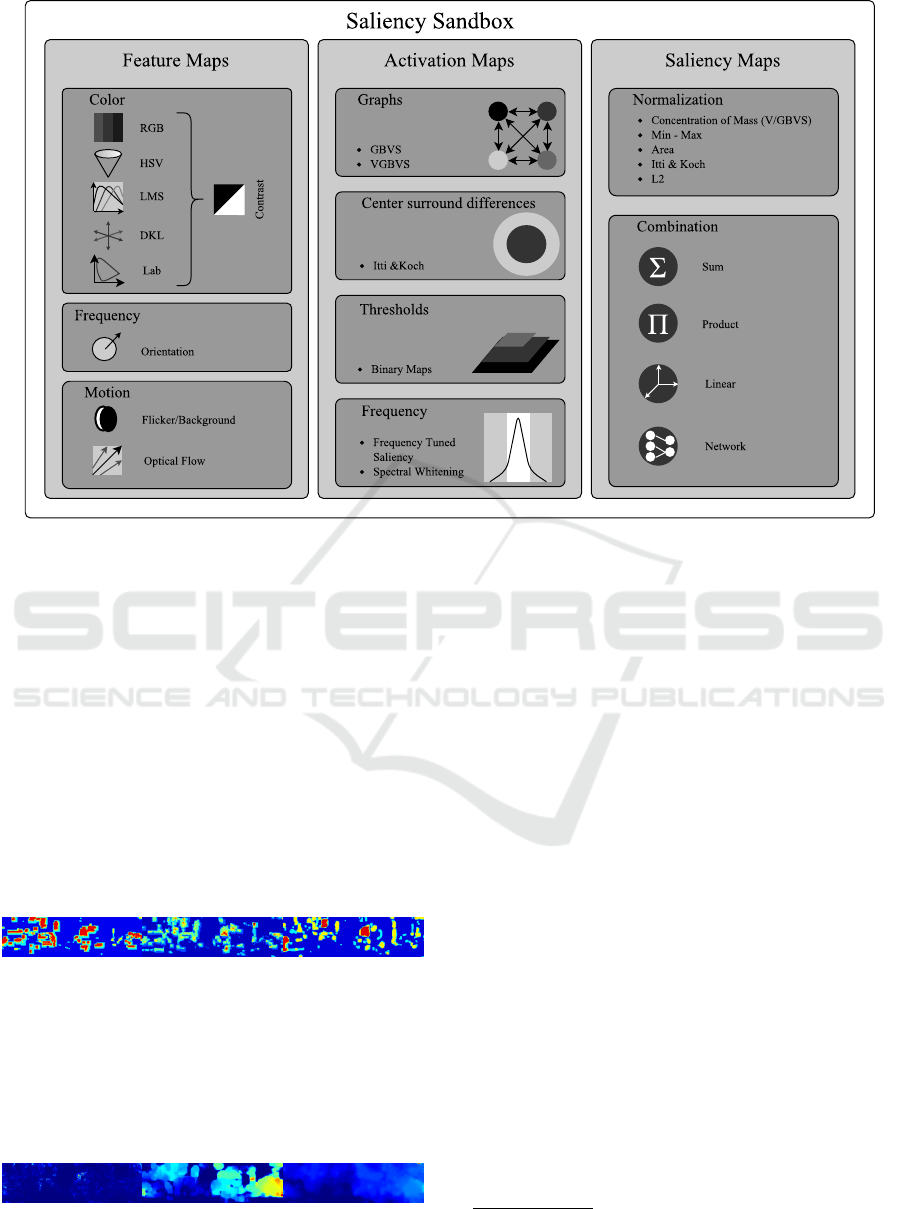
Figure 4: The Saliency Sandbox provides various types of features and activation maps. The color features are based on the
actual color value of a pixel, while the orientation is extracted by applying Gabor filters. The motion class provides feature
extractors based on sequential images. Activation maps extract the saliency in a single feature map. We already implemented
some of the best-known approaches such as the GBVS, the center surround differences provided by Itti & Koch, Boolean
Maps based on different levels of thresholding, and the Frequency Tuned Saliency or Spectral Whitening as frequency based
approaches. All activation maps can be applied to all features which leads to a high number of possible combinations.
Different kinds of activation maps can be combined to one saliency map.
background subtraction to extract motion features
from sequential images. MOG
f
and MOG2
f
employ
Gaussian mixture models to describe the distribution
of a background pixel over a sequence of images. The
probable values of a pixel are those more static over
the sequence (KaewTraKulPong and Bowden, 2002;
Zivkovic, 2004). The GMG
f
background subtraction
uses a Bayesian model to detect foreground objects
(Godbehere et al., 2012).
MOG
f
(I
i
, I
i−1
) MOG2
f
(I
i
, I
i−1
) GMG
f
(I
i
, I
i−1
)
Optical Flow: As a further motion feature, the
Saliency Sandbox provides several optical flow
algorithms. The optical flow is high pass filtered
to reduce the influence of ego-motion, especially
in driving scenes. Ego-motion is estimated by a
polynomial whereby recent images in the sequence
are weighted higher than older ones.
Brox
f
(I
i
, I
i−1
) Farneback
f
(I
i
, I
i−1
) TV L1
f
(I
i
, I
i−1
)
3.2 Activation Models
Activation models emphasize salient regions based on
a feature map. The Saliency Sandbox offers five dif-
ferent activation models whereby each of them uses
fundamentally different approaches.
GBVS: The GBVS is inspired by the retinotopically
organized network in the visual cortex. It creates a
transition matrix from each pixel to all others. The
transition weight is defined by the dissimilarity of
two pixels and the distance
3
of their location in the
image. Used as a Markov model, the activation is
calculated by iterative multiplication with an initial
equally distributed vector (Harel et al., 2006a). Con-
sidering the quadratic size of the transition matrix,
the input feature usually needs to be downscaled
massively. In this example, the input was downscaled
to 32 × 32 pixels. Processing videos, GBVS comes
with the advantage that the previous activation can
be used as the initial value for the Markov system,
which reduces the number of necessary iterations
significantly. GBVS normalizes the activation by a
3
The edge is weighted higher, the closer the distance be-
tween pixels.
Saliency Sandbox - Bottom-up Saliency Framework
661
concentration of the masses. For this, a transition
matrix is created again but with the activation and
distance as transition weights. The Markov system is
solved just as above (Harel et al., 2006a).
GBV S
a
(L + M) GBV S
a
(L − M) GBVS
a
(S − (L + M))
Itti & Koch: The approach by (Itti and Koch,
2000) uses center surround differences to model
the receptive field of a sensory neuron. The center
surround differences are implemented as a pyramid
of different input scales. Subtracting the feature maps
of two different scales results in a high response
if a feature was noticeable in the higher scaled but
not in the lower scaled feature map. Itti & Koch
suggest an iteratively applied DoG filter followed by
a rectification for normalization (Itti and Koch, 2000).
Itti
a
(L + M) Itti
a
(L − M) Itti
a
(S − (L + M))
Boolean Maps: In contrast to the other activation
maps, Boolean Maps emphasize salient features in
the global image. A number of random thresholds
is applied to the feature map. The resulting binary
maps are collected along with their complements.
After applying morphological opening operations to
remove noise and not enclosed objects, the binary
maps are summed up (Zhang and Sclaroff, 2013). In
our implementation, the thresholds are not generated
randomly as this makes the result hard to compare
and unstable in image sequences. Instead, we spread
a fixed number of thresholds evenly between the
minimum and maximum value in the feature map.
The normalization is realized by an L2-normalization.
BM
a
(L + M) BM
a
(L − M) BM
a
(S − (L + M))
Frequency Tuned: The Frequency Tuned Saliency
calculates the Euclidean distance between the Lab
color value of a Gaussian filtered input and the av-
erage Lab color value (Achanta et al., 2009). Since
the average color value is calculated over the whole
image, the Frequency Tuned Saliency is a global
saliency detection, similarly to the Boolean maps. In-
stead of the average color, we use a heavily low-pass
filtered image in our implementation. Thus, our im-
plementation is also able to detect saliency in a local
context of the image. We also removed the calcula-
tion of the Euclidean distance over the channels since
we apply the activation on each channel separately.
If we set σ
2
= ∞ for the second low pass filter, and
calculate the activation FT
a
(I) for each channel
in the Lab color space, we just have to calculate
p
FT
a
(L)
2
+ FT
a
(a)
2
+ FT
a
(b)
2
as the composition
step to comply with the original implementation.
FT
a
(L + M) FT
a
(L − M) FT
a
(S − (L + M))
Spectral Whitening: This frequency based ap-
proach from (Hou and Zhang, 2007) was reimple-
mented based on the Spectral Saliency Toolbox from
(Schauerte and Stiefelhagen, 2012). It analyzes
the log spectrum of the input image to obtain the
spectral residual and transform it to a spatial domain
to achieve the saliency map.
S
f
(L + M) S
f
(L − M) S
f
(S − (L + M))
3.3 Composite
The activation of several features is usually combined
to one saliency map. All methods implemented in the
Saliency Sandbox use weighted sums for the combi-
nation of activation maps. Other approaches such as
linear weights or neural networks are not included yet.
GBVS: The GBVS combines color features as
luminance, red-green, and blue-yellow together with
orientation features. The activation is calculated in
different scales and combined by the mean over all of
them. As default, the implementation from J. Harel
uses the DKL colorspace, corresponding to the last
example below (Harel et al., 2006b).
GBV S
RGB
GBV S
Lab
GBV S
DKL
Itti & Koch: Itti & Koch use seven activation maps.
The first three calculate the center surround differ-
ences in the red-green, blue-yellow, and intensity
feature map. As the GBVS, the Itti & Koch map
uses four orientation features (0
◦
, 45
◦
, 90
◦
, 135
◦
).
They propose the red-green and blue-yellow pseudo
channels extracted from an RGB input (corresponds
to the first example) (Itti and Koch, 2000).
Itti
s RGB
Itti
s Lab
Itti
s DKL
Boolean Maps: (Zhang and Sclaroff, 2013) use the
Lab color channels as features and combine them by
calculating the mean over the three activation maps.
BM
s RGB
BM
s Lab
BM
s DKL
Frequency Tuned: The Frequency Tuned Saliency
was designed as a band pass filter in the Lab
color space (Achanta et al., 2009). As previously
mentioned, the original implementation uses the
VISAPP 2017 - International Conference on Computer Vision Theory and Applications
662

Euclidean distance to composite the activation map
of each color channel to one saliency map. The
examples below show the result by just summing the
activation maps.
FT
s RGB
FT
s Lab
FT
s DKL
Spectral Whitening: The color space is not spec-
ified in the work by (Hou and Zhang, 2007). The
implementation in the Spectral Saliency Toolbox
provided by (Schauerte and Stiefelhagen, 2012)
calculates the mean of the normalized activation map
from each color channel if there is more than one
channel. The examples below show the result of this
procedure created by the Saliency Sandbox based on
different color spaces.
S
s RGB
S
s Lab
S
s DKL
Mixed The Mixed saliency model was created to
demonstrate the flexibility of the Saliency Sandbox.
It combines activations based on Spectral Whitening,
Itti & Koch, Boolean Maps and Farneback motion.
Mix
s RGB
Mix
s Lab
Mix
s DKL
4 USAGE
One of our major goals is to speed up research by pro-
viding a framework that covers a huge set of features,
activations, and utilities to run them. Furthermore,
the framework should be fast and easily extendable to
implement new approaches. In the following, we pro-
vide three code snippets that demonstrate how new
functionalities can be added and applied.
Define New Activation: The following snippet
shows how a new activation map can be defined.
The related feature is passed as a template argument.
The base class Saliency derives from class Algorithm
which was already introduced in section 2. Default
parameters are defined in the reset function, which
is called by the abstract base whenever the algorithm
should be reset. The actual calculation of the activa-
tion is placed in the calc function.
te m p l at e<
u i n t 1 6 t wi d t h , / / i n p u t / o u t p u t wi d t h
u i n t 1 6 t h e i g h t , / / i n p u t / o u t p u t h e i g h t
te m p l at e<u i n t 1 6 t , u i n t 1 6 t >typename f e a t u r e / / f e a t u r e t y p e
>
c l a s s M y A c t i v a t i o n S a l i e n c y : p u b l i c S a l i e n c y< w i d t h , h e i g h t >{
p r i v a t e :
f e a t u r e < w i d t h , h e i g h t > m f e a t u r e ;
p u b l i c :
v o i d r e s e t ( ) {
t h i s −>s e t S t r i n g ( ” t e x t ” , ” ” ) ; / / s e t d e f a u l t
}
v o i d c a l c ( ) {
/ / do s o m e t h i n g w i t h t h e p r o p e r t y
s t d : : c o u t << t h i s −>g e t S t r i n g ( ” t e x t ” ) << s t d : : e n d l ;
/ / c a l c u l a t e t h e f e a t u r e map
t h i s −>m f e a t u r e . p r o c e s s ( t h i s −>i n p u t ( ) ) ;
/ / c a l c u l a t e t h e o u t p u t
t h i s −>o u t p u t (
/ / c a l c u l a t e t h e a c t i v a t i o n map
a c t i v a t e ( t h i s −>m f e a t u r e . o u t p u t ( ) )
) ;
} ;
Combine Activation Maps: To combine multiple
activation maps into a saliency map, the following
snippet declares the class MySaliency deriving from
SumSaliency. The activation maps are passed as tem-
plate arguments and will be invoked by the Sum-
Saliency parallel using a thread pool. The activation
results will be summed up in the output buffer. Sum-
Saliency derives from the Algorithm base class and
is therefore also usable in Matlab and Simulink. The
abstract function setParams is called in the reset func-
tion and allows to configure the individual activation
maps.
te m p l at e<
u i n t 1 6 t wi d t h , / / i n p u t / o u t p u t wi d t h
u i n t 1 6 t h e i g h t / / i n p u t / o u t p u t h e i g h t
>
c l a s s My S al i en c y : p u b l i c S u m Sa l ien c y< w i d t h , h e i g h t ,
/ / I t t i & Koch a c t i v a t i o n on a DKL c o l o r f e a t u r e
I t t i S a l i e n c y < w i d t h , h e i g h t , D KLC o lo r S al i enc y >,
/ / New d e f i n e d a c t i v a t i o n
M y A c t i v a t i o n S a l i e n c y< wi d t h , h e i g h t , D K L Co l orS a lie n cy>
> {
p u b l i c :
v o i d s e t P a r a m s ( u i n t 1 6 t i n d e x , s a l t ∗ s a l ) {
s w i t c h ( i n d e x ) {
c a s e 0 :
/ / u s e t h e f i r s t d k l c h a n n e l ( L−M) a s f e a t u r e
/ / f o r t h e I t t i & Koch a c t i v a t i o n
s a l −>s e t I n t ( ” d k l . c h a n n e l ” , 1 ) ;
br e ak ;
c a s e 1 :
/ / M y A c t i v a t i o n S a l i e n c y s h o u l d s a y h e l l o
s a l −>s e t S t r i n g ( ” t e x t ” , ” h e l l o w o r l d ” ) ;
br e ak ;
}
}
} ;
Create a Tool: After creating an own activation map
and a new composition with a Itti & Koch activation,
this last example shows how an executable is created
to examine a video for saliency.
i n t main ( i n t ar g c , c o n s t c h a r ∗ a r g v [ ] ) {
MyS a l ienc y<RES HD> s a l ;
/ / p r i n t h e l p
f o r ( i n t i = 1 ; i < a r g c ; i ++)
i f ( ! s t r c m p ( a r g v [ i ] , ”−−h e l p ” ) | | ! st r c m p ( a r g v [ i ] , ”−h ” ) )
s a l . p r i n t P a r a m s ( ) ;
a l g o r i t h m a s s e r t ( a r g c >= 3 ) ;
/ / p a r s e a l g o r i t h m p a r a m e t e r s
s a l . p a r s e P a r a m s ( a r g c −3,& a r g v [ 3 ] ) ;
/ / p r o c e s s v i d e o
s a l . p r o c e s s V i d e o ( a r g v [ 1 ] , a r g v [ 2 ] ) ;
r e t u r n 0 ; }
Saliency Sandbox - Bottom-up Saliency Framework
663

5 FINAL REMARKS
The Saliency Sandbox is still under development and
grows continuously in terms of available feature and
activation maps. Further, we will add functional-
ity for evaluation based on real gaze data. By inte-
grating algorithms for eye movement detection (e.g.
MERCY (Braunagel et al., 2016)) and scanpath anal-
ysis (e.g., SubsMatch (K
¨
ubler et al., 2014)) in dy-
namic scenes, we will creating a basis for further ex-
tensions such as the explorative search for suitable
combinations of activation and feature maps or neu-
ral networks for a non-linear combination of activa-
tion maps. Here, the focus is primarily on dynamic
scenes instead of single frames, which evokes new
challenges since there are only few gaze points per
frame available. The goal is to create a comprehen-
sive environment in order to implement new saliency
maps quickly and comparable or to combine existing
approaches to design saliency maps for a particular
use case.
Source code, binaries for Linux x64, and extensive
documentation are available at:
www.ti.uni-tuebingen.de/perception
REFERENCES
Achanta, R., Hemami, S., Estrada, F., and Susstrunk, S.
(2009). Frequency-tuned salient region detection.
In IEEE conference on Computer vision and pattern
recognition, 2009. CVPR 2009., pages 1597–1604.
Braunagel, C., Geisler, D., Stolzmann, W., Rosenstiel, W.,
and Kasneci, E. (2016). On the necessity of adap-
tive eye movement classification in conditionally au-
tomated driving scenarios. In Proceedings of the Ninth
Biennial ACM Symposium on Eye Tracking Research
& Applications, pages 19–26. ACM.
Derrington, A. M., Krauskopf, J., and Lennie, P. (1984).
Chromatic mechanisms in lateral geniculate nucleus
of macaque. The Journal of Physiology, 357(1):241–
265.
Godbehere, A. B., Matsukawa, A., and Goldberg, K.
(2012). Visual tracking of human visitors under
variable-lighting conditions for a responsive audio art
installation. In 2012 American Control Conference
(ACC), pages 4305–4312. IEEE.
Harel, J., Koch, C., and Perona, P. (2006a). Graph-based vi-
sual saliency. In Advances in neural information pro-
cessing systems, pages 545–552.
Harel, J., Koch, C., and Perona, P. (2006b). A saliency im-
plementation in matlab. URL: http://www. klab. cal-
tech. edu/˜ harel/share/gbvs. php.
Hou, X. and Zhang, L. (2007). Saliency detection: A spec-
tral residual approach. In 2007 IEEE Conference on
Computer Vision and Pattern Recognition, pages 1–8.
IEEE.
Itti, L. (2004). The iLab Neuromorphic Vision C++ Toolkit:
Free tools for the next generation of vision algorithms.
The Neuromorphic Engineer, 1(1):10.
Itti, L. and Koch, C. (2000). A saliency-based search mech-
anism for overt and covert shifts of visual attention.
Vision Research, 40(10):1489–1506.
ITU (2011). Studio encoding parameters of digital televi-
sion for standard 4:3 and wide screen 16:9 aspect ra-
tios.
KaewTraKulPong, P. and Bowden, R. (2002). An im-
proved adaptive background mixture model for real-
time tracking with shadow detection. In Video-based
surveillance systems, pages 135–144. Springer.
Kasneci, E., Kasneci, G., K
¨
ubler, T. C., and Rosenstiel, W.
(2015). Online recognition of fixations, saccades, and
smooth pursuits for automated analysis of traffic haz-
ard perception. In Artificial Neural Networks, pages
411–434. Springer.
K
¨
ubler, T. C., Kasneci, E., and Rosenstiel, W. (2014). Sub-
smatch: Scanpath similarity in dynamic scenes based
on subsequence frequencies. In Proceedings of the
Symposium on Eye Tracking Research and Applica-
tions, pages 319–322. ACM.
Patrone, A. R., Valuch, C., Ansorge, U., and Scherzer,
O. (2016). Dynamical optical flow of saliency
maps for predicting visual attention. arXiv preprint
arXiv:1606.07324.
Schauerte, B. and Stiefelhagen, R. (2012). Quaternion-
based spectral saliency detection for eye fixation pre-
diction. In Computer Vision–ECCV 2012, pages 116–
129. Springer.
Tafaj, E., Kasneci, G., Rosenstiel, W., and Bogdan, M.
(2012). Bayesian online clustering of eye movement
data. In Proceedings of the Symposium on Eye Track-
ing Research and Applications, ETRA ’12, pages
285–288. ACM.
Treisman, A. M. and Gelade, G. (1980). A feature-
integration theory of attention. Cognitive psychology,
12(1):97–136.
Von Goethe, J. W. (1840). Theory of colours, volume 3.
MIT Press.
Walther, D. and Koch, C. (2006). Modeling attention to
salient proto-objects. Neural networks, 19(9):1395–
1407.
Zhang, J. and Sclaroff, S. (2013). Saliency detection: A
boolean map approach. In Proceedings of the IEEE
International Conference on Computer Vision, pages
153–160.
Zivkovic, Z. (2004). Improved adaptive gaussian mixture
model for background subtraction. In Pattern Recog-
nition, 2004. ICPR 2004. Proceedings of the 17th In-
ternational Conference on, volume 2, pages 28–31.
VISAPP 2017 - International Conference on Computer Vision Theory and Applications
664
