
Hex-utils: A Tool Set Supporting HexASCII Hexagonal rasters
Lu
´
ıs Moreira de Sousa and Jo
˜
ao Paulo Leit
˜
ao
Eawag - Swiss Federal Institute of Aquatic Science and Technology,
¨
Uberlandstrasse 133, 8600 D
¨
ubendorf, Switzerland
Keywords:
HexASCII, Hexagonal raster, Hexagonal Mesh, Hex-utils.
Abstract:
The advantages of hexagonal meshes over squared grids in discretising spatial variables have been known
for long. Notwithstanding, the raster data formats used in geo-spatial disciplines to this purpose are still
today almost exclusively reliant on squared grids. The HexASCII file format is a core element in an attempt
to introduce hexagonal rasters to mainstream GIS, defining a simple vehicle to store and share such data
structures. This article describes the hex-utils tool-kit, an Application Programming Interface (API) and a
set of command line tools enabling the use of HexASCII rasters. Basic operations are supported: creation
of new hexagonal rasters from different inputs and transformation into file formats readable by desktop GIS
programmes. The API sets a framework for the development of further functionality.
1 INTRODUCTION
In Geographic Information Systems (GIS), the raster
data structure provides a straightforward mean to cap-
ture real world phenomena, by discretising spatial
variables into tessellations of samples. Rasters divide
the cartographic plane regularly into small areas of
the same shape, inside which the spatial variable in
question is assumed to be constant. This is possible
only with three regular geometric shapes (i.e., hav-
ing all sides of equal length): the equilateral triangle,
the square and the hexagon. Raster grids used in GIS
have been predominantly organised in squared pat-
terns in which the space between each row and each
column of samples is constant; to a good extent this is
a consequence of spatial data acquisition methods.
However, hexagonal rasters yield two essential
advantages over square grids that are relevant in GIS.
In first place is the higher spatial resolution pro-
vided by hexagonal meshes of equal area (Mersereau,
1979); or conversely, the lower number of cells re-
quired by a hexagonal raster to match the resolu-
tion of a squared counterpart. In second place is the
isotropy of the hexagonal neighbourhood; in a square
grid each cell has four neighbours to which it shares
an edge and four with which it shares only a vertex.
In a hexagonal raster each cell shares an edge with
each of its six neighbours, and all their cell centroids
are at the same distance.
On the downside, hexagons yield the distinc-
tive characteristic of not being dividable into smaller
hexagons, and neither forming a larger hexagon when
agglomerated. This issue has been addressed in dif-
ferent ways, such as that proposed with the Gener-
alised Balanced Ternary cell index system (Gibson
and Lucas, 1982). Moreover, raster cell aggregation
is not a frequent operation in spatial analysis pro-
cesses.
The shortcomings of square grids became evident
early in the history of Computer Science, motivat-
ing suggestions for a shift to hexagonal meshes al-
ready in 1960s (Golay, 1969). But in spite of further
theoretical developments and other advantages iden-
tified, this shift never fully materialised. Likewise in
the GIS field, neither hexagonal raster file formats,
nor supporting tools were ever fully developed. Scant
work with hexagonal sampling schemes or hexagonal
meshes is conducted on vector topologies.
These were the motivations leading to the specifi-
cation of the HexASCII file format (HASC for short),
an open formalism to store and port hexagonal rasters
as text files (de Sousa and Leit
˜
ao, In review). This
specification sets the minimum information required
to capture cell geometry, mesh dimensions and loca-
tion, plus the cell data themselves.
A prototype application is presented in this article,
a set of tools developed to provide basic functional-
ity for HexASCII rasters. It comprises an Applica-
tion Programming Interface (API) and a set of com-
mand line tools demonstrating the creation of Hex-
ASCII rasters and their integration with existing GIS
software. These assets intend to be a step towards the
Sousa, L. and Leitão, J.
Hex-utils: A Tool Set Supporting HexASCII Hexagonal rasters .
DOI: 10.5220/0006275801770183
In Proceedings of the 3rd International Conference on Geographical Information Systems Theory, Applications and Management (GISTAM 2017), pages 177-183
ISBN: 978-989-758-252-3
Copyright © 2017 by SCITEPRESS – Science and Technology Publications, Lda. All rights reserved
177

adoption of hexagonal rasters in GIS and spatial anal-
ysis practice.
These tools are gathered in a project called
hex-utils released under an open source licence and
made available at GitHub
1
. They can also be installed
from a PyPi repository
2
.
This article starts with a brief overview of the Hex-
ASCII file format in Section 2; Section 3 describes
the API underlying the tool-kit and Section 4 goes
through the various command line tools developed to
date; Section 5 summarises the article and points to
future work.
2 OVERVIEW OF THE HexASCII
FILE FORMAT
An HexASCII raster is a text file composed by two
parts: an opening metadata section and a string of cell
values. The metadata section describes cell and mesh
geometry and positions the raster in the cartographic
domain. The metadata is described with a set of seven
key and value pairs, of which five are mandatory and
two are optional:
• ncols: number of columns;
• nrows: number of rows;
• xll: x coordinate of the lower left cell centroid;
• yll: y coordinate of the lower left cell centroid;
• side: cell side length;
• angle: mesh rotation angle (optional);
• no data: string representing null or missing val-
ues (optional).
Listing 1 presents the HexASCII file for the
hexagonal raster depicted in Figure 1. The full spec-
ification of this file format, as well as the reasoning
leading to its structure, is available in (de Sousa and
Leit
˜
ao, In review).
Listing 1: Example of an HexASCII file.
ncols 4
nrows 3
xll 3.1
yll 2.2
side 2
angle 15
no_da t a 9999
11 21 31 41
12 22 32 42
13 23 33 43
1
https://github.com/ldesousa/hex-utils
2
https://pypi.python.org/pypi/hex-utils
132.2
3.1
2
15º
O
11
21
31
41
12
22
32
42
43
33
23
Figure 1: The hexagonal raster described by the HASC file
in Listing 1.
3 THE HexASCII APPLICATION
PROGRAMMING INTERFACE
(API)
The tools enabling the HexASCII file format were de-
veloped in the Python programming language (Sanner
et al., 1999). This language was chosen in first place
for its versatility, as useful to ad hoc scripting as to
high level object-oriented programming. Python also
facilitates the manipulation of spatial data through a
number of libraries such as GDAL/OGR (Warmer-
dam, 2008) OWSLib
3
, Shapely
4
or GeoPandas
5
,
granting it growing popularity among geo-spatial pro-
grammers.
The prototype command line tools rely on the do-
main model depicted in Figure 2, describing rasters
in general and then specific file formats. This domain
model is the blueprint for the API implemented in the
Python programming language. Both the HexASCII
format and the ASCII squared raster format specified
by ESRI
6
are included in this model. The latter is one
of the data sources for the creation of new hexagonal
rasters.
The model starts with the abstract class Grid that
encloses various aspects of a raster. This class can be
seen as a template for the minimum metadata, data
and functionality required for a raster grid format.
3
https://geopython.github.io/OWSLib/
4
https://pypi.python.org/pypi/Shapely
5
http://geopandas.org/
6
http://resources.esri.com/help/9.3/arcgisdesktop/com/
gp toolref/spatial analyst tools/esri ascii raster format.htm
GISTAM 2017 - 3rd International Conference on Geographical Information Systems Theory, Applications and Management
178
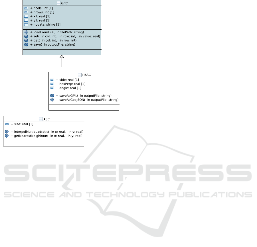
Figure 2: The domain model underlying the tools support-
ing the HASC file format.
These include: number of columns (ncols), number
of rows (nrows), coordinates positioning the grid in
the cartographic space (xll and yll) and an identi-
fier for empty or null values (nodata). The data is
stored internally as a two-dimensional array, that can
not be directly assessed (it is a protected property).
The init() method initialises the properties de-
scribed above in a child instance of the Grid class.
To assign a new value to a grid cell there is the set()
method, that takes as arguments a column number, a
row number and a new value. Conversely, to retrieve
the value of a cell, there is the get() method, tak-
ing as arguments a column and a row number. The
loadFromFile() method provides the functionality
to read the raster metadata and data from an existing
file. Finally, the save() method is available to cre-
ate a persistent file on disk with the current data and
metadata of the instance, according to the format sub-
scribed to by the child class.
The ASC class is a concrete implementation of the
Grid type, representing the ESRI ASCII raster for-
mat. Beyond the properties inherited from Grid, this
class adds the size property, another metadata ele-
ment determining the width and height of each grid
cell. The init() method is redefined to allow the set
up of this additional property. Two new methods are
introduced in this class, both concerning the interpo-
lation of data values: (i) getNearestNeighbour(),
that simply returns the value of the cell whose cen-
troid is nearest to the given coordinates, and (ii)
interpolMultiquadratic(), that for a given pair
of coordinates applies the multi-quadratic interpola-
tion technique (Chaplot et al., 2006) with the values
of the nine nearest cells. These methods are used to
interpolate grid values for a resulting HexASCII type
grid.
Lastly there is the HASC class, the concrete imple-
mentation of the HexASCII file format. It adds three
properties: (i) side - the length of an hexagonal cell
side; (ii) hexPerp - the distance between two paral-
lel sides of a cell; and (iii) angle - the angle of ro-
tation of the grid. The hexPerp property is required
in various calculations (e.g. cell area, cell centroids),
thus it keeps the value at hand avoiding its constant
computation. An important difference from the ESRI
ASCII raster file format to HexASCII is grid posi-
tioning. While in the HexASCII format the positional
coordinates (the xll and yll properties) refer to the
centre of the lower left cell, in the ESRI format these
coordinates refer to the lower left corner of the lower
left cell.
The HASC class also introduces a few meth-
ods. The init() method is again redefined
to set up the class specific properties. The
getCellCentroidCoords() method returns the car-
tographic location of a cell, given its discrete coordi-
nates (column and row). The saveAsGML() method
persists the mesh instance as a vector file using
the Geography Markup Language (GML) (Burggraf,
2006), a standard maintained by the Open Geospatial
Consortium (OGC). This method creates an hexag-
onal polygon for each grid cell, to which is as-
signed an attribute named value with the respec-
tive cell value. A similar output is produced by the
saveAsGeoJSON() method, but producing a vector
file using the GeoJSON language (Butler et al., 2008).
4 COMMAND LINE TOOLS
Using the API described above, a number of com-
mand line tools are made available with hex-utils to
perform basic operations with HexASCII grids; each
one is detailed below.
4.1 asc2hasc
This tool provides a simple mean to create an hexag-
onal raster from an existing square raster. It
calculates the geometry of the resulting hexagonal
mesh and uses either the nearest neighbour or the
multi-quadratic interpolation techniques to calculate
Hex-utils: A Tool Set Supporting HexASCII Hexagonal rasters
179

its values (using the getNearestNeighbour() and
interpolMultiquadratic() methods of the ASC
class).
The asc2hasc tool functions in two distinctive
modes: either preserving cell area (using the -a flag)
or preserving spatial resolution (-r flag). In the first
mode the resulting hexagonal cells are conceived to
have the same area of the original squares; this means
a larger number of cells in the resulting hexagonal
mesh. In the -r mode the resulting hexagonal cells
are 13.4% larger than the original squares. This last
mode does not preserve entirely the same spatial res-
olution, since the interpolation itself induces a certain
loss of signal detail. From this hexagonal cell area pa-
rameter is derived the hexagonal cell side (S
h
), a key
element in the ensuing calculations.
The following step is the computation of the num-
ber of columns and rows in the resulting mesh. The
number of columns is calculated as the minimum
number that can entirely cover the horizontal span of
the grid, as given in the following expression:
C
h
=
C
s
S
s
3S
h
/2
(1)
Where C
h
is the number of columns in the hexag-
onal grid, C
s
the number of columns in the square
grid, S
s
the side of the input square cells and S
h
the
side of the resulting hexagonal cells. 3S
h
/2 is the dis-
tance between two opposite vertices of the hexagonal
cell. The application of the ceiling operation guaran-
tees that all square cells are covered in the horizontal
sense.
This computation is not as straightforward for the
number of rows, since there is a vertical displace-
ment of 3S
h
/2 between two consecutive columns in a
North-South hexagonal grid (where two sides of each
hexagon are parallel to the xx axis). To save space, the
option in this case is to cover only partially the input
square cells at the bottom row; the number of rows is
thus calculated as follows:
R
h
=
R
s
S
s
√
3S
h
(2)
Where R
h
is the number of rows in the hexagonal
mesh and R
s
the number of rows in the square grid.
The resulting mesh is positioned in space with the
number of rows in mind. Even columns are set in
order to cover exactly the top square row; odd rows
thus miss partially the bottom square row. This bot-
tom sleave uncovered by odd rows is at most
√
3S
h
/4
in height. The concrete coordinates of the lower left
hexagonal centroid are thus computed as:
x0
h
= x0
s
+ S
h
/2 (3)
Rs Ss -
Rh √3 Sh +
√3 Sh / 2
Sh / 2
Figure 3: Positioning of an HASC grid relative to the square
grid of origin.
y0
h
= y0
s
+ R
s
S
s
−R
h
√
3S
h
+
√
3S
h
/2 (4)
Where the pair (x0
s
,y0
s
) are the coordinates of the
lower left corner of the square grid and (x0
h
,y0
h
) the
centroid coordinates of the lower left hexagonal cell.
Figure 3 exemplifies these calculations.
The resulting hexagonal mesh covers as much
as possible of the original square without exceed-
ing exaggeratedly the original extent. This option
“by excess” means extra extents along the margins
of the original grid. The top half of the top cells in
odd columns and part of the bottom of cells in even
columns lay beyond the extent of the original grid
7
.
The leftmost column can exceed the original extent
by as much as 3S
h
/2.
Beyond the arguments determining cell dimen-
sions, the asc2hasc tool takes also the -m flag defin-
ing which interpolation technique to use. Two options
are available: mq for multi-quadratic interpolation and
nn for the nearest neighbour. Finally, the flags -i and
-o provide the paths to the input ESRI ASCII square
raster and the output HexASCII file. An example of
use:
asc2hasc -r -m mq -i /path/to/input.asc
-o /path/to/output.hasc
4.2 csv2hasc
This tool creates a new HexASCII raster from a set of
point samples. This is a common operation in GIS, in
which users extrapolate a regular mesh over a region
of interest from a collection of sparsely located ob-
servations. Spatial variables subject to such treatment
may be temperature, rainfall, altitude, soil quality, etc.
7
Note that grid indexing starts with zero, e.g. the left-
most cell columns in Figure 3 are even.
GISTAM 2017 - 3rd International Conference on Geographical Information Systems Theory, Applications and Management
180

The basic input to the tool is a comma separated
values (CSV) file (Shafranovich, 2005), structured
in three columns representing in succession: easting
coordinate, northing coordinate and observed value.
Each row corresponds to an individual observation.
Listing 2 provides an example.
Listing 2: Example of a CSV file input to csv2hasc.
1002.5 , 845.2 ,57.3 ,
1005.1 , 850.7 ,66.2 ,
998.6 ,841.9 , 4 2 . 7 ,
1007.2 , 852.4 ,38.9 ,
The user must also declare an area of interest to
be covered by the resulting raster. This is particularly
useful if the observations do not cover exactly the re-
gion under study. Additionally, the desired cell geom-
etry must be specified too. These inputs are provided
to the tool through a set of arguments:
-x : the bottom x coordinate of the area of interest.
-y : the left y coordinate of the area of interest.
-X : the top x coordinate of the area of interest.
-Y : the right y coordinate of the area of interest.
-s : the length of the cell side in the resulting grid.
-i : path to the input CSV file.
-o : path to the output HASC raster file.
The output hexagonal mesh is dimensioned and
positioned in the Cartographic space using the same
process described in Section 4.1 and exemplified in
Figure 3. The values of the new HexASCII raster
are interpolated using the multi-quadratic method, ap-
plied to the five samples closest to each cell centroid.
An example of usage:
csv2hasc -x 0 -y 0 -X 2000 -Y 2000
-s 0.62 -i input.csv -o output.hasc
4.3 surface2hasc and
surface2asc
In order to assess the comparative performance of
hexagonal and square rasters of similar spatial res-
olution two tools where developed that sample di-
rectly a given continuous surface. With these tools
a same method or process can be applied on equiv-
alent rasters to investigate different results between
hexagons and squares. Sampling directly a continu-
ous surface avoids the signal losses that would occur
interpolating from an existing raster or from a set of
sparse observations.
As their name imply, surface2hasc produces an
HexASCII raster and surface2asc an ESRI ASCII
grid. They require a series of inputs that declare the
spatial extent to sample, the geometry of the resulting
mesh and identify the location of the surface function.
Each of these inputs is provided with a specific argu-
ment:
-x : the bottom x coordinate of the extent to sample.
-y : the left y coordinate of the extent to sample.
-X : the top x coordinate of the extent to sample.
-Y : the right y coordinate of the extent to sample.
-s : the length of the cell side in the resulting grid.
-m : the Python module containing the surface func-
tion.
-f : the name of the surface function.
-o : path to the output raster file.
The tool starts by calculating cell geometry and
then positions a mesh overlapping the extent declared.
In the hexagonal case the same “by excess” approach
employed in the asc2hasc tool is applied. The sur-
face function is then imported; it is assumed it resides
in a reachable Python module, declared with the -m
argument. The function is assumed to take in two ar-
guments, the easting and northing coordinates, and to
return a numerical value
8
. Figure 4 presents an exam-
ple surface and the resulting HexASCII grid produced
with the following command:
surface2hasc -x 0 -y 0 -X 2000 -Y 2000
-s 19.6 -m surfaces.surfaceGaussian
-f fun -o output.hasc
4.4 hasc2gml and hasc2geojson
The hasc2gml tool creates a GML file representing
the input HexASCII raster. For each cell of the raster
a polygon feature is created in the GML file with its
exact geometry. To each feature is assigned an at-
tribute named value containing the value of the corre-
sponding HexASCII cell. The resulting GML file is
usually thirty times larger than the original HexAS-
CII, stressing the usefulness of the latter as a portable
file format.
hasc2gml uses directly the loadFromFile() and
saveAsGML() methods of the HASC class. It takes no
additional arguments, beyond the paths to the input
and output files. The following exemplifies its use:
hasc2gml /path/to/input.hasc
/path/to/output.gml
8
A few surface examples are available at the GitHub
repository, in the surfaces package.
Hex-utils: A Tool Set Supporting HexASCII Hexagonal rasters
181
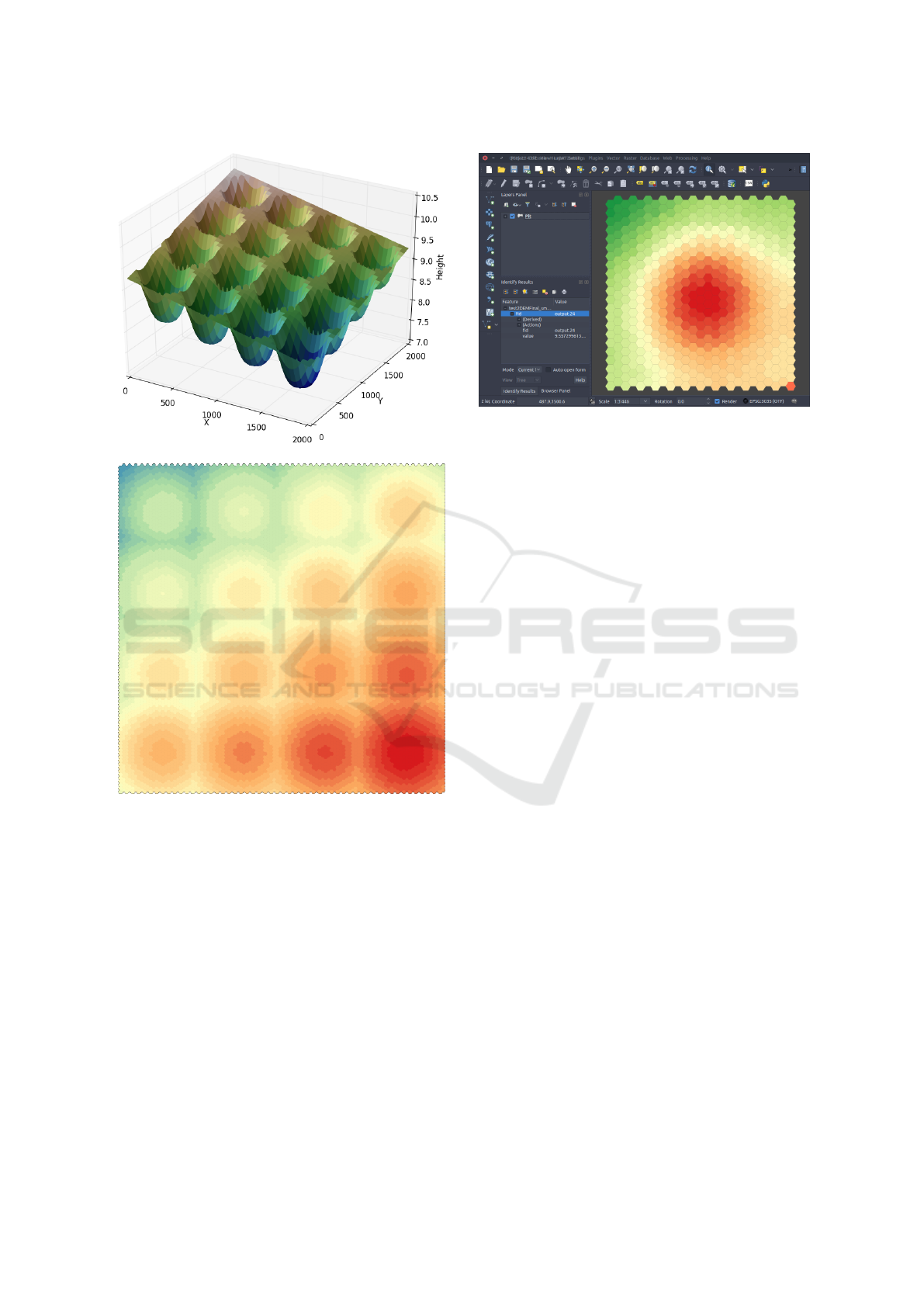
(a) Continous surface.
(b) HASC displayed as a GML layer in QGIS.
Figure 4: A sample surface and the resulting HASC grid
displayed in QGIS.
The hasc2geojson tool is in all similar, with
the difference being the output data format, GeoJ-
SON (Butler et al., 2008) in this case. This data for-
mat requires in general one third less disk space than
GML; still it requires some twenty times the space
used by the original HexASCII.
hasc2geojson /path/to/input.hasc
/path/to/output.json
The purpose of these tools is to facilitate the
visualisation of HexASCII grids in traditional GIS
desktop software. The resulting GML or GeoJSON
files can be seamlessly loaded into one of such pro-
grammes and there be subject to styling with choro-
Figure 5: An HASC raster displayed through a GML layer
in QGIS.
pleths, feature selection, feature inquiring, geometri-
cal assessment and so forth. Figure 5 portraits a GML
file created from an HexASCII raster displayed in
QGIS (Team et al., 2013).
5 SUMMARY AND FUTURE
WORK
In spite of their well known advantages over tradi-
tional square grids, hexagonal rasters are yet to be
adopted as a common data structure in GIS. Such
evolution is unlikely to happen without tools facili-
tating the use of this space partitioning pattern. The
hex-utils tool-kit is a first step in this direction, to-
wards the ultimate goal of making hexagonal meshes
as easy to use as their squared counterparts in GIS.
The hex-utils tool-kit comprises a basic API
and a set of command line tools providing essential
functionality to manipulate HexASCII rasters. They
make possible the creation of hexagonal rasters and
their visualisation in desktop GIS software. The API
can be the basis for the development of further soft-
ware supporting hexagonal rasters.
The next steps towards a simplified use of hexago-
nal rasters will have to address data acquisition, with
mechanisms to translate other common spatial data
sources into hexagonal rasters. Tools to transform
LiDAR point clouds or to discretise vectors into Hex-
ASCII rasters are therefore natural extensions to the
hex-utils tool-kit. Another step concerns the devel-
opment of hexagonal map algebra tools; a prototype
previously developed in the C# language (de Sousa,
2006) is a candidate to be integrated into the tool-kit.
Modern GIS software has become increasingly
easy to evolve and extend. The development of ad-
GISTAM 2017 - 3rd International Conference on Geographical Information Systems Theory, Applications and Management
182

vanced tools and data structures, such as hex-utils
and the HexASCII file format, is today not only sim-
pler, but also easier to reach by a wide range of poten-
tial users. All elements seem to be in place for hexag-
onal rasters to finally start entering the mainstream
GIS.
REFERENCES
Burggraf DS. 2006. Geography markup language. Data Sci-
ence Journal. 5:178–204.
Butler H, Daly M, Doyle A, Gillies S, Schaub T,
Schmidt C. 2008. The geojson format specification.
URL: http://wwwgeojsonorg/geojson-spechtml/ (ac-
cessed 29-11-2016).
Chaplot V, Darboux F, Bourennane H, Legu
´
edois S, Sil-
vera N, Phachomphon K. 2006. Accuracy of interpo-
lation techniques for the derivation of digital elevation
models in relation to landform types and data density.
Geomorphology. 77(1):126–141.
de Sousa LM. 2006.
´
Algebra de Mapas em Grelhas Hexag-
onais [master’s thesis]. Universidade T
´
ecnica de Lis-
boa.
de Sousa LM, Leit
˜
ao JP. In review. HexASCII: a file for-
mat for cartographical hexagonal rasters. International
Journal of Geographic Information Science.
Gibson L, Lucas D. 1982. Spatial data processing using
generalized balanced ternary. In: Proceedings of the
IEEE Conference on Pattern Recognition and Image
Processing. p. 566–571.
Golay MJE. 1969. Hexagonal parallel pattern transforma-
tions. IEEE Transactions on Computers. 18(8):733–
740.
Mersereau R. 1979. The processing of hexagonally sampled
two-dimensional signals. In: Proceedings of the IEEE;
Vol. 67. p. 930–949.
Sanner MF, et al. 1999. Python: a programming lan-
guage for software integration and development. J
Mol Graph Model. 17(1):57–61.
Shafranovich Y. 2005. Common format and mime
type for comma-separated values (csv) files. URL:
https://2rfcnet/4180 (accessed 13-02-2017).
Team QD, et al. 2013. Qgis geographic information sys-
tem. Open Source Geospatial Foundation Project
http://qgis osgeo org.
Warmerdam F. 2008. The geospatial data abstraction li-
brary. In: Open source approaches in spatial data han-
dling. Springer; p. 87–104.
Hex-utils: A Tool Set Supporting HexASCII Hexagonal rasters
183
