
Time Weight Content-based Extensions of Temporal Graphs
for Personalized Recommendation
Armel Jacques Nzekon Nzeko’o
1,2,3
, Maurice Tchuente
1,2
and Matthieu Latapy
3
1
Sorbonne Universités, UPMC Université Paris 06, IRD, UMI 209 UMMISCO, F-93143, Bondy, France
2
CETIC, Université de Yaoundé I, Faculté des Sciences, Departement d’Informatique, BP 812, Yaoundé, Cameroon
3
Sorbonne Universités, UPMC Université Paris 06, CNRS, UMR 7606, LIP6, F-75005, Paris, France
Keywords: Temporal Recommendation, Long- and Short-term Preferences, Session-based Temporal Graph, Time
Weight Content-based Graph, Time-averaged Hit Ratio, PageRank, Injected Preference Fusion.
Abstract: Recommender systems are an answer to information overload on the web. They filter and present to
customers, small subsets of items that they are most likely to be interested in. Users’ interests may change
over time, and accurately capturing this dynamics in such systems is important. Sugiyama, Hatano and
Yoshikawa proposed to take into account the user’s browsing history. Ding and Li were among the first to
address this problem, by assigning weights that decrease with the age of the data. Others authors such as
Billsus and Pazzani, Li, Yang, Wang and Kitsuregawa proposed to capture long- and short- terms
preferences and combine them for personalized search or news access. The Session-based Temporal Graph
(STG) is a general model proposed by Xiang et al. to provide temporal recommendations by combining
long- and short-term preferences. Later, Yu, Shen and Yang have introduced Topic-STG, which takes into
account topics information extracted from data. In this paper, we propose Time Weight Content-based STG
that generalizes Topic STG. Experiments show that, using Time-Averaged Hit Ratio as measure, this time
weight content-based extension of STG leads to performance increases of 4%, 6% and 9% for CiteUlike,
Delicious and Last.fm datasets respectively, in comparison to STG.
1 INTRODUCTION
The amount of information in web sites like
Amazon, Netflix and Last.fm is considerable and
fast-growing. For users, browsing and searching in
such data has become very difficult. To solve this
problem, recommender systems filter and present to
customers, small subsets of items that they are most
likely to be interested in.
Early recommender systems did not take into
account temporal information (Herlocker et al.,
1999). This is strong limitation because user’s
profiles and context evolve with time. In this regards
Sugiyama et al., (2004) proposed to adapt results
according to time-evolving user profiles, based for
instance on browsing history. Ding and Li (2005)
were among the first to take time explicitly into
account by assigning decreasing weights according
to their age. Later, some authors proposed to capture
both long- and short-term preferences and combine
them for recommendations (Billsus and Pazzani,
2000; Li et al., 2007).
Interest in temporal recommender systems
increased considerably since the 2009 Netflix grand
prize (Koren, 2009). Koren’s solution was based on
a dataset with items rated by users, whereas in
practice, data often contains the history of users in
terms of their interactions with items. For instance,
Last.fm offers datasets in which each line indicates
the fact that user u listened to song i at time t.
In this line of research, Xiang et al., (2010)
propose Session-based Temporal Graphs (STG),
which model long- and short-term preferences
separately. However, they ignore features of items,
and so they miss for instance the fact that interest in
a piece of music is related to its author. In order to
improve this, Yu et al., (2014) extend the STG into
Topic-STG for personalized tweet recommendation.
They add topic nodes to the STG and link tweets to
their topics.
These recommender graphs process edges
regardless of their age. This fails to capture the fact
that in most situation, recent transactions are the
most likely to reflect user preferences in the near
268
Nzeko’o, A., Tchuente, M. and Latapy, M.
Temporal Recommendation, Long- and Short-term Preferences, Session-based Temporal Graph, Time Weight Content-based Graph, Time-averaged Hit Ratio, PageRank, Injected Preference
Fusion..
DOI: 10.5220/0006288202680275
In Proceedings of the 13th International Conference on Web Information Systems and Technologies (WEBIST 2017), pages 268-275
ISBN: 978-989-758-246-2
Copyright © 2017 by SCITEPRESS – Science and Technology Publications, Lda. All rights reserved

future (Ding and Li, 2005). For example, the clothes
that a boy wears have great variability related to his
age, thus, the impact of his past dress style on his
future dress style decreases with time. To take this
into account, we propose here to weight edges
according to their age, so that older edges have
lower influence. We propose the Time Weight
Content-based STG, in which edges are labelled
with their last occurrence time, and we use an
exponential decay function proposed by Ding and Li
(2005) to weight edges accordingly.
The remaining of this paper is organized as
follow: Section 2 presents Session-based Temporal
Graphs and the two recommendation algorithms,
PageRank (Page et al., 1999) and Injected
Preference Fusion (IPF) (Xiang et al., 2010) on
which our work is built. Section 3 introduces the
Time Weight Content-based STG model. Section 4
is devoted to experiments. We discuss related work
in Section 5, and we summarize our findings in
Section 6.
2 BACKGROUND
We use the notations and definitions proposed by
Xiang et al., (2010), together with some additional
concepts related to content and time, summarized in
Table 1.
2.1 Session-based Temporal Graph
We consider data under the form of a link stream,
i.e. a set of triples (t, u, i) representing the fact that
user u has selected item i at time t. For each user u
(resp. each item i), we define user node v
u
(resp. item
node v
i
). We denote by T the time span of the
dataset and we divide T into time slices of equal
duration. For each of these slices T, we define
session node v
u,T
. A session is not defined here as a
time slice during which the user interacts with the
system. It rather corresponds to a time slice during
which a user has a specific behaviour.
A session-based temporal graph G(U, S, I, E, w)
is a directed bipartite graph with three types of
nodes: U is the set of user nodes, S the set of session
nodes and I the set of item nodes. The function
w: E R is a non-negative weight function for
edges. The set of edges, E, is obtained as follows.
For each triplet (t, u, i), let us consider T the time
slice to which t belongs. Then, E contains edges
(v
u
, v
i
) and (v
i
, v
u
), which represent long-term
preference between user u and item i; and E contains
Table 1: Notations and definitions.
Symbol
Description
G
bipartite graph STG
CG
bipartite graph Content-based STG
TG
bipartite graph Time weight Content-
based STG
E
edge set in any graph
V
set of all nodes in any graph
U, I, S, C
user node set, item node set, session
node set, content node set
v
u
, v
i
, v
u,T
, v
c
user node, item node, session node,
content node
w
weight function defined on STG edges
w
C
weight function defined on Content-
based STG edges
w
T
time weight function defined on Time
weight Content-based STG edges
v
k
, v
k+1
propagation function of IPF from
v
k
to v
k+1
out v
out node set of the node v
parameter to control the preference
propagation
dose of long-term preference injected
to user node
parameter to adjust the edge weight
from item nodes to user/session nodes
c
parameter to control the influence of
content features in the preference
propagation
parameter used to compute the time
weight function
damping factor for PageRank
personalization
(v
u,T
, v
i
) and (v
i
, v
u,T
), which represent short-term
preferences.
The weight function is defined as:
(1)
In (1),
u
models the influence of long-term
preferences and
s
models the influence of short-
term preferences. To simplify the model, we can use
u
̸
s
for
u
and 1 for
s
Fig. 1 is an example of STG with 3 user nodes, 5
session nodes, 7 item nodes and 2 time slices. It
shows that user u
1
has selected items i
1
, i
2
, user u
2
has selected items i
3
, i
4
and user u
3
has selected item
i
5
during the first time slice T
1
. During the second
time slice T
2
, user u
1
has selected i
3
and user u
3
has
selected i
6
and i
7
.
Temporal Recommendation, Long- and Short-term Preferences, Session-based Temporal Graph, Time Weight Content-based Graph,
Time-averaged Hit Ratio, PageRank, Injected Preference Fusion.
269

Figure 1: Example of STG.
2.2 Temporal Personalized Random
Walk
The Temporal Personalized Random Walk (TPRW)
(Xiang et al., 2010) is a personalization of the
PageRank algorithm defined by Page et al. (Page et
al., 1999) for nodes ranking in graphs. It was defined
to tackle temporal recommendation using the idea of
Haveliwala (Haveliwala, 2002). It corresponds to the
following formula:
PR = M PR (1 ) d (2)
where is the damping factor, M is a transition
matrix and vector d is a user-specific personalized
vector indicating which nodes the random walker
will jump to after a restart.
When making recommendations for user u,
vector d favors user node v
u
and the most recent
session node v
u,T
as follows:
(3)
In other words, long-term preferences are injected to
user node v
u
and short-term preferences are injected
to session node v
u,T
through vector d.
When we implement the PageRank with iterative
power law method, we stop when the difference of
two consecutives rank vectors is of norm less than or
equal to a threshold .
2.3 Injected Preference Fusion
The IPF algorithm is an extension of the random
walk with injection of preferences and customization
of preference propagation. To recommend items to a
user u, the algorithm proceeds in 3 steps:
Injection of long-term preferences
on the user
node v
u
and injection of short-term preferences (1
) on the most recent session node v
u,T
of user
u.
Propagation of preferences by random walk of
length 3 on the graph according to the formula.
(4)
where out(v
k
) denotes the set of out-neighbors of
node v
k
,
is a parameter used to tune the
propagation process, w(v
k
, v
k+1
) is the weight of
arc (v
k
, v
k+1
) and
(v
k
, v
k+1
) is the proportion of
preference of v
k
that is propagated to v
k+1
.
Recommendation of Top-N items that have
received the greatest preference values and that
user u has not yet selected.
The IPF random walk length is limited to 3
following experimental result (Xiang, et al., 2010).
3 TIME WEIGHT CONTENT-
BASED EXTENSIONS OF STG
In this section, we first illustrate how to construct
Content-based STG (CSTG) which is similar to
Topic-STG (Yu et al., 2014). We end by showing
how to construct Time Weight Content-based STG
(TCSTG).
3.1 Content-based Session-based
Temporal Graph
The basic STG model neglects item properties which
can contain significant information for the prediction
of user’s behaviour. This motivated Phuong et al.,
(2008) to add to the user-item bipartite graph, new
nodes corresponding to content. The same idea is
applied here to obtain Content-based STG.
To construct the Content-based STG, we need to
have item properties in our data, so we don’t use a
set of triples like in the construction of STG. We
rather use a set of quadruples (t, u, i, c) where t, u
and i have the same meaning as in STG, and c is a
content feature of i.
Content-based STG CG(U, S, I, C, E, w
C
) is a
directed graph obtained from the STG G(U, S, I, E,
w) by adding for any link (t, u, i, c), the six
additional arcs (v
u
, v
c
), (v
c
, v
u
), (v
u,T
, v
c
), (v
c
, v
u,T
),
WEBIST 2017 - 13th International Conference on Web Information Systems and Technologies
270

(v
i
, v
c
) and (v
c
, v
i
). With respective weights 1,
, 1,
1,
c
,
c
as illustrated in Fig. 2.
Figure 2: Edge weights in content-based STG.
3.2 Time Weight Content-based
Session-based Temporal Graph
The Content-based STG neglects the ages of edges
when assigning weights. So, it cannot capture the
evolution of users’ interest which we assume to be
sensitive to time as suggested by Ding and Li
(2005). The recommendation model presented here
assigns a greater weight to recent edges and lower
weight to older edges. More precisely, the weight of
the arc (v, v’) is defined by:
(5)
where w(v, v’) is the weight in the graph without
time weight, t is the most recent time at which edge
(v, v’) appears and f(t) is a time-dependent decay
function as in (Ding and Li, 2005). Here we take
(6)
where is the decay rate and (t
r
– t) is the difference
in second between time t
r
at which we are making
recommendations and t.
The parameter can also be defined as
0
where
0
is the delay after which the weight of an
edge reduces by 1/2.
0
is also called half life
parameter.
4 EXPERIMENTS
We have conducted a set of experiments to examine
the performance of Time weight Content-based
STG. For each model, we consider various values of
parameters and we retain the best performance. We
also implemented the classic bipartite user-item
graph (BIP) to show the effects of taking into
account long- and short-term preferences in graph
models.
The experiment environment is as follow: the
executions of our programs are done using a
computer with 64GB of RAM and 16 processors
Intel of 2.93GHz and 4MB of cache. For
implementation, we have used the Python 2.7
language and the Networkx 1.11 module for graph
manipulation. Note that we have changed the
Networkx PageRank in order to stop when
convergence is not reached after 100 iterations. We
used SQLite 3 as DBMS and Matplotlib 1.4.0 to
produce graphics.
4.1 Data Description
Following the example of Xiang et al, our goal is to
make recommendations based on implicit data from
various real world domains. To this effect, we first
perform experiments on the social bookmarking
datasets CiteUlike and Delicious (Cantador et al.,
2011) which were used in (Xiang et al., 2010). This
provides a good basis for the evaluation of the
improvement obtained when temporal aspects are
taken into account. We also use data from Lastfm
(Celma, 2010), a web site where users can listen to
music because in this domain the fashion effect
plays an important role with the consequence that,
the impact of past tastes on the future ones decreases
with time.
We model our data as link streams {(t, u, i, c)},
where any quadruple has different interpretation
depending on domains. In the case of CiteUlike and
Delicious, each quadruplet means that user u has
bookmarked page i at time t with tag c. And for the
Last.fm data, this means that user u has listened to
song i at time t and c is the author of i.
Before modeling our data as link streams, we
performed a filtering by ignoring items and users
that did not appear a number of times higher than a
given threshold
. Table 2 provides details on our
data: date of the first link, date of the last link, total
duration of link streams, threshold used, number of
users, number of items, number of content features
and number of links.
Table 2: Data statistics.
Start date
End date
Duration
CiteUlike
2010-01-01
2010-07-02
183 days
10
Delicious
2010-05-11
2010-11-09
183 days
7
Last.fm
2005-02-14
2005-08-16
183 days
8
Users
Items
Content
Links
CiteUlike
1318
424
4216
16885
Delicious
894
298
2789
13825
Last.fm
135
1054
225
41604
Temporal Recommendation, Long- and Short-term Preferences, Session-based Temporal Graph, Time Weight Content-based Graph,
Time-averaged Hit Ratio, PageRank, Injected Preference Fusion.
271

4.2 Experiment and Evaluation
The evaluation process is done periodically as in (Li
and Tang, 2008) and (Lathia et al., 2009). Before
starting experiments, we have to divide the link
streams into time windows of a fixed length . We
fix to 15 days because humans live at a monthly
pace, and the first 15 days are generally
characterized by consumption behaviours just after
getting salary, that are different from the ones
observed during the last 15 days of the month. To
simplify the experimentation process, we adopt the
same as the length of session when constructing
STG. Here after, N denotes the number of time
slices.
For each time window W
k
, for k=1,..,N-1, we
proceed as follows:
Construct the graphs corresponding to data of W
1
,
W
2
, .. ,W
k.
.
Compute the Top-N recommendations for users
who have selected at least one “new item” during
the time window W
k+1
.
Evaluate the algorithm by computing the ratio of
users for which at least one of these Top-N items
recommends has been selected during W
k+1
. This
proportion is also call Hit Ratio
(Karypis,
2001).
After determining the Hit Ratio for each window,
compute the Time Averaged Hit Ratio (TAHR) that
is a weighted combination of the N-1 values
obtained above for the Hit Ratio. The weight of each
Hit Ratio
is the number of corresponding
users
as in the following equation:
(7)
Note that, although the convergence may be very
slow for some examples, we have noticed that, in
most cases, the convergence is achieved after at
most 100 iterations.
4.3 Exploration of the Range of the
Parameters
Let us see how the parameters are obtained in
Table 3. We proceed as in (Xiang et al., 2010). The
parameters correspond to the vector [
0,
,
,
c
,
,
], whose components are numbered 1, 2, 3, 4, 5, 6
from left to right. This vector is initialized to
[0, 0.5, 0.5, 0.5, 0.5, 0.5]. Then, we consider the
values of
0 shown in the second row of Table 3,
while maintaining the other parameters at their
initial value 0.5. We perform ten experiments and
take for
0 the value corresponding to the best
performance. For instance we obtain for
0 the
interval [7, 30] for TPRW-TCSTG in CiteUlike
dataset as shown in Table 4. Given this optimal
value for
0 we then give to the eleven successive
values shown in the third row of Table 3, while
maintaining the other parameters at their initial
value. We obtain for the interval [0.4, 1] for
TPRW-TCSTG in CiteUlike dataset as shown in
Table 4. This process is repeated for the remaining
parameters.
Figure 3 shows all the variations of Time-
Averaged Hit Ratio with parameter values in the
case of CiteUlike. The complete set of parameters
explored is shown in Table 3 and the best values
obtained with this procedure are shown in Table 4.
Table 3: Parameters values.
Parameters
Initial
value
Set of values
0 (in days)
0
0, 1, 7, 15, 30, 45, 60, 90, 180, 365
0.5
0.1 × i for i = 0..10
0.5
0, 0.1, 0.2, 0.3, 0.4, 0.5, 0.6, 0.7, 0.8, 0.9, 1,
1.5, 3, 5, 10, 15, 20, 30, 50, 100
c
0.5
0, 0.1, 0.2, 0.3, 0.4, 0.5, 0.6, 0.7, 0.8, 0.9, 1,
1.5, 3, 5, 10, 15, 20, 30, 50, 100
0.5
0.1 × i for i = 0..10
0.5
0.1 × i for i = 0..10
4.4 Accuracy Comparison
The performances of PageRank and IPF applied to
STG, Time-weight content-based STG, Content-
based STG and classical bipartite graph, for the three
datasets are presented in Table 5. It can be seen that
PageRank applied to the Time weight content-based
STG gives the best results, followed by Content-
based STG. Moreover, STG is always better than the
classical bipartite graph, which confirms the
relevance of STG.
Moreover, for PageRank applied to the Time
weight content-based STG, the optimal value of the
half life parameter
0, is less than one month for
social bookmarking dataset, but is greater than one
month for music dataset. This may be due to the fact
that the impact of web pages that someone consulted
in the past on those that he is likely to consult in the
future decreases very quickly with time. On the
contrary, tastes are more stable for music and the
impact of a past music does not decrease very
quickly.
WEBIST 2017 - 13th International Conference on Web Information Systems and Technologies
272
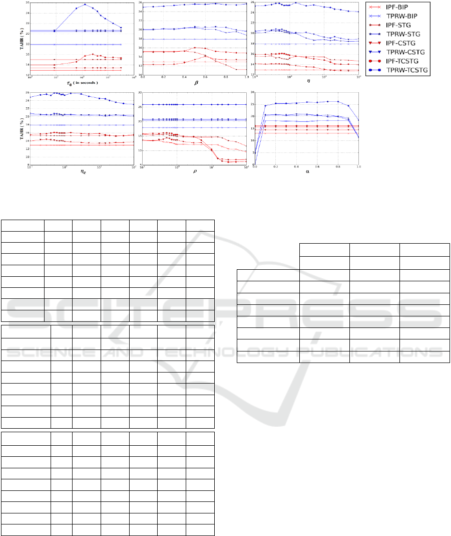
Figure 3: Variation of Time Averaged Hit Ratio with parameter values in the case of CiteUlike.
Table 4: Best parameter values.
CiteUlike
0
c
IPF-BIP
-
-
-
-
0.1-0.3
-
IPF-STG
-
0.0-0.5
0.1-0.3
-
0.1-0.7
-
IPF-CSTG
-
0.5-1
0.0-0.9
0.2-0.5
0.5-0.6
-
IPF-TCSTG
15-60
0.5-0.6
0.1-0.9
0.4-1.5
0.1-1
-
TPRW-BIP
-
-
-
-
-
0.1-0.9
TPRW-STG
-
0.0-0.7
0.3-0.6
-
-
0.1-0.7
TPRW-CSTG
-
0.5-0.8
0.3-0.6
0.1-0.7
-
0.1-0.6
TPRW-TCSTG
7-30
0.4-1
0.3-1.5
0.5-3
-
0.5-0.8
Delicious
0
c
IPF-BIP
-
-
-
-
0.1-10
-
IPF-STG
-
0.0-0.4
0-0.1
-
0.1-0.6
-
IPF-CSTG
-
0.5
15-50
0.3-0.9
0.4-1.5
-
IPF-TCSTG
1-7
0.5-0.6
0.5-0.8
50-100
0.5-1.5
-
TPRW-BIP
-
-
-
-
-
0.1-0.9
TPRW-STG
-
0.0-0.4
0.1-0.2
-
-
0.2-0.5
TPRW-CSTG
-
0.0-0.6
15-100
0.2-0.8
-
0.5-0.7
TPRW-TCSTG
7
0-1
0.5-0.8
0-0.1
-
0.1-04
Last.fm
0
c
IPF-BIP
-
-
-
-
0.1-0.8
-
IPF-STG
-
0.5-1
0.9-1.5
-
1.5-10
-
IPF-CSTG
-
0-0.4
0-0.3
30-100
0.4-0.6
-
IPF-TCSTG
1-15
0-0.4
0.1-0.3
1-100
10-50
-
TPRW-BIP
-
-
-
-
-
0.1-0.5
TPRW-STG
-
0.5-0.7
0.1-1.5
-
-
0.2-0.5
TPRW-CSTG
-
0.2-0.4
0.2-0.5
5-30
-
0.4-0.6
TPRW-TCSTG
30-90
0.5-0.7
0.4-0.6
1-5
-
0.4-0.7
We also think that PageRank has better
performance because in this algorithm the
propagation process is not limited to the proximity
of the source node as in IPF. Indeed PageRank also
favours the recommendation of the most popular
items of the graph because, even when they are far
from the source node, they can be reached and then
have a great influence thanks to their high degree.
Table 5: Performances for the best parameters.
CiteUlike
Delicious
Last.fm
TAHR (%)
TAHR (%)
TAHR (%)
IPF-BIP
13.5
7.3
16.3
IPF-STG
15.7
8.6
18.2
IPF-CSTG
14.4
6.4
28.9
IPF-TCSTG
16.1
9.7
26.6
TPRW-BIP
18.3
8.8
27.9
TPRW-STG
20.6
9.2
30.2
TPRW-CSTG
20.9
10.7
37.7
TPRW-TCSTG
26.1
13.2
38.9
5 RELATED WORK
In this section, we present some work on time aware
recommender systems followed by recommender
systems that use item properties. Finally, we present
some graph-based recommender systems.
5.1 Time Aware Recommender
Systems
Ding et al. (Ding and Li, 2005) propose the use of an
exponential decay function to assign greater weights
to latest ratings when computing similarities in
collaborative filtering. Subsequently, Liu et al.,
(2010) have proposed an incremental collaborative
filtering where one decay function is used to
compute similarities and another one is used for
prediction. Recently, Karahodža et al., (2015)
assumed that the importance of interest granted to an
item decreases in a similar manner for similar users.
Some recommender systems are based on the
Temporal Recommendation, Long- and Short-term Preferences, Session-based Temporal Graph, Time Weight Content-based Graph,
Time-averaged Hit Ratio, PageRank, Injected Preference Fusion.
273

assumption that importance of information is
ephemeral. Thus, Lathia et al., (2009) set a time
window size, then, any information is used during
one time slice and ignored at the next time window.
Such recommender systems only capture short-term
preferences.
Some studies are not based only on short-term
preferences but also consider that importance of
some information persists over time (Li et al., 2007).
The STG model (Xiang et al., 2010) extends this
work but ignores item properties.
5.2 Content-based Recommender
Systems
The content-based recommender systems seek to
recommend similar items to the one the user already
like. As Lops et al. (Lops et al., 2011) argue, the
basic idea is to match features associated to users’
preferences and items so as to recommend new
items that address their needs. This approach is
already used in various domains such as books
recommendation on Amazon website based on their
description (Mooney and Roy, 2000), and web pages
recommendation (Pazzani et al., 1996).
Although content-based recommender systems
can propose items that have not already been
purchased in the past, it is also useful to use user
similarities by combining this approach with
collaborative filtering techniques. Indeed,
Balabanovic and Shoham (1997) and Basu et al.,
(1998) show that the combination of collaborative
filtering and content-based filtering may result in a
recommender system that eliminates the weaknesses
of both approaches. In this paper, we have used a
graph model to realize this combination.
5.3 Graph based Recommender
Systems
The simplest graph-based recommender systems
only use user-item links. A bidirectional edge is
created between a user node and an item node if the
user has purchased the concerned item. Finally, an
item is recommended to a user if the user has not yet
purchased that item and if there is a path from the
user to that item. The most used recommender
algorithms on the graphs are based on the random
walk (Baluja et al., 2008), like PageRank and IPF
which are used in this paper.
The use of graph paths to recommend new items
can be seen as collaborative filtering where
similaritys defined through node distance. However,
such recommender graphs do not take into
consideration item properties. To remedy this
limitation, Phuong et al., (2008) have constructed a
recommender graph in which they have added a
third node type: the type “content”. The obtained
recommender system is actually a combined
collaborative filtering and content-based filtering.
The associated graph ignores the temporal aspect of
data and therefore cannot accurately capture short-
and long-term preferences. Yu et al., (2014) propose
the Topic-STG which combines those two
preferences and takes into account topics related to
tweets. However, those models handle edges
regardless of their age. This is not in accordance
with concept drift. This is why we propose a new
extension of STG where edge weights are decreased
using a time decay function as in (Li and Tang,
2008).
6 CONCLUSIONS
This paper proposes time weight content-based
extensions of the temporal graph model introduced
by Xiang et al., As in Topic-STG introduced by Yu,
Shen and Yang, we represent content by nodes, but
we penalize older interactions. Experiments show
that, using Time-Averaged Hit Ratio as measure,
this time weight content-based extension of STG
leads to performance increases of 4%, 6% and 9%
for CiteUlike, Delicious and Last.fm datasets
respectively, in comparison to STG. This gives
evidence of the fact that the age of interactions is a
relevant feature for recommender systems.
More experiments using datasets from various
domains are needed in order to adjust the length of
time windows and other parameters.
ACKNOWLEDGEMENTS
This work is funded in part by the African Center of
Excellence in Information and Communication
Technologies (CETIC), the UPMC-IRD PDI
program, by the European Commission H2020
FETPROACT 2016-2017 program under grant
732942 (ODYCCEUS), by the ANR (French
National Agency of Research) under grants ANR-
15-CE38-0001 (AlgoDiv) and ANR-13-CORD-
0017-01 (CODDDE), by the French program "PIA-
Usages, services et contenus innovants" under grant
O18062-44430 (REQUEST), and by the Ile-de-
France program FUI21 under grant 16010629
(iTRAC).
WEBIST 2017 - 13th International Conference on Web Information Systems and Technologies
274

REFERENCES
Balabanović, M., & Shoham, Y. (1997). Fab: content-
based, collaborative recommendation.
Communications of the ACM , 40 (3 ), 66-72.
Baluja, S., Seth, R., Sivakumar, D., Jing, Y., Yagnik, J.,
Kumar, S., et al. (2008, April). Video suggestion and
discovery for youtube: taking random walks through
the view graph. In Proceedings of the 17th
international conference on World Wide Web. ACM ,
895-904.
Basu, C., Hirsh, H., & Cohen, W. (1998, July).
Recommendation as classification: Using social and
content-based information in recommendation. In
Proceedings of the fifteenth national/tenth conference
on Artificial intelligence/Innovative applications of
artificial intelligence , 714-720.
Billsus, D., & Pazzani, M. J. (2000). User modeling for
adaptive news access. User modeling and user-
adapted interaction , 10 (2-3), 147-180.
Cantador, I., Brusilovsky, P., & Kuflik, T. (2011). 2nd
Workshop on Information Heterogeneity and Fusion
in Recommender Systems (HetRec 2011). In
Proceedings of the 5th ACM conference on
Recommender systems .
Celma, Ò. (2010). Music Recommendation and Discovery
in the Long Tail. Springer.
Ding, Y., & Li, X. (2005, October). Time Weight
Collaborative Filtering. In Proceedings of the 14th
ACM international conference on Information and
knowledge management, ACM , 485-492.
Haveliwala, T. H. (2002, May). Topic-sensitive pagerank.
In Proceedings of the 11th international conference on
World Wide Web , 517-526.
Herlocker, J. L., Konstan, J. A., Borchers, A., & Riedl, J.
(1999). An algorithmic framework for performing
collaborative filtering. In : Proceedings of the 22nd
annual international ACM SIGIR conference on
Research and development in information retrieval.
ACM.
Karahodža, B., Donko, D., & Šupić, H. (2015, May).
Temporal Dynamics of Changes in Group Users
Preferences in Recommender Systems. In 38th
International Convention on Information and
Communication Technology, Electronics and
Microelectronics, IEEE , 1262-1266.
Karypis, G. (2001, October). Evaluation of Item-Based
Top-N Recommendation Algorithms. In Proceedings
of the tenth international conference on Information
and knowledge management , 247-254.
Koren, Y. (2009). The bellkor solution to the netflix grand
prize. Netflix prize documentation , 81, 1-10.
Lathia, N., Hailes, S., & Capra, L. (2009, July). Temporal
Collaborative Filtering With Adaptive
Neighbourhoods. In Proceedings of the 32nd
international ACM SIGIR conference on Research and
development in information retrieval, ACM , 796-797.
Li, L., Yang, Z., Wang, B., & Kitsuregawa, M. (2007).
Dynamic adaptation strategies for long-term and short-
term user profile to personalize search. In Advances in
Data and Web Management , 228-240.
Li, Y., & Tang, J. (2008). Expertise Search in a Time-
varying Social Network. In The Ninth International
Conference on Web-Age Information Management,
IEEE , 293-300.
Liu, N. N., Zhao, M., Xiang, E., & Yang, Q. (2010).
Online Evolutionary Collaborative Filtering. In
Proceedings of the fourth ACM conference on
Recommender systems. ACM , 95-102.
Lops, P., De Gemmis, M., & Semeraro, G. (2011).
Content-based recommender systems: State of the art
and trends. In Recommender systems handbook.
Springer US , 73-105.
Mooney, R. J., & Roy, L. (2000, June). Content-based
book recommending using learning for text
categorization. In Proceedings of the fifth ACM
conference on Digital libraries , 195-204.
Page, L., Brin, S., Motwani, R., & Winograd, T. (1999,
November). The PageRank citation ranking: bringing
order to the web. Technical Report, Stanford InfoLab .
Pazzani, M., Muramatsu, J., & Billsus, D. (1996). Syskill
& Webert: Identifying interesting web sites. In
Proceedings of the thirteenth American Association
for Artificial Intelligence AAAI/IAAI , 1, 54-61.
Phuong, N. D., Thang, L. Q., & Phuong, T. M. (2008). A
Graph-Based Method for Combining Collaborative
and Content-Based Filtering . In Trends in Artificial
Intelligence. Springer Berlin Heidelberg , 859-869.
Sugiyama, K., Hatano, K., & Yoshikawa, M. (2004, May).
Adaptive web search based on user profile constructed
without any effort from users. In Proceedings of the
13th international conference on World Wide Web,
ACM , 675-684.
Xiang, L., Yuan, Q., Zhao, S., Chen, L., Zhang, X., Yang,
Q., et al. (2010). Temporal recommendation on graphs
via long-and short-term preference fusion. In :
Proceedings of the 16th ACM SIGKDD international
conference on Knowledge discovery and data mining.
ACM , 723-732.
Yu, J., Shen, Y., & Yang, Z. (2014). Topic-STG :
Extending the Session-based Temporal Graph
Approach for Personalized Tweet Recommendation.
In Proceedings of the companion publication of the
23rd international conference on World wide web
companion. International World Wide Web
Conferences Steering Committee , 413-414.
Temporal Recommendation, Long- and Short-term Preferences, Session-based Temporal Graph, Time Weight Content-based Graph,
Time-averaged Hit Ratio, PageRank, Injected Preference Fusion.
275
