
Derivation of Real Driving Emission Cycles based on Real-world
Driving Data
Using Markov Models and Threshold Accepting
Roman Liessner, Robert Fechert and Bernard Bäker
Dresden Institute of Automobile Engineering, TU Dresden, George-Bähr-Straße 1c, 01069 Dresden, Germany
Keywords:
Driving Cycle, Real Driving Emissions, RDE, Markov Model, Threshold Accepting.
Abstract:
The European Union has decided to bring the Real Driving Emissions (RDE) law into force in 2016. From this
point onward, the air pollutants a vehicle emits under real driving conditions will be measured by means of a
so-called Portable Emissions Measurement System (PEMS) and then used as the basis for licensing. Compared
to the emission values presently determined in the New European Driving Cycle (NEDC), a significant rise can
be expected. This change is on the one hand caused by a substantially more dynamic driving style prescribed
by RDE regulations, and on the other hand by considerably larger variations of ambient conditions. A trend
of development resulting from this conversion is the creation of test cycles conforming to RDE regulations,
which enable vehicle development to adhere to the new licensing regulations. The validity of a RDE drive is
gradually verified based on multiple criteria before respective emission values are determined at the end of
the process. The contribution at hand presents a new approach for generating RDE substitute cycles. At first,
the criterion of driving dynamics will be focussed upon. To realize this, combinatorics of a large set of real
driving data will be used to generate substitute cycles, which will exhibit driving dynamics as high as possible.
This specification achieves universal, vehicle independent limitation cycles featuring high emission levels. By
using the described limitation cycles, a first vehicle examination concerning the fulfilment of RDE regulations
is made possible.
1 INTRODUCTION
Because of the ongoing emission discrepancies be-
tween homologation measurement and real driving
measurement, the European Union has decided to
bring Real Driving Emission (RDE) tests for type test-
ing into force in January of 2016. The mentioned dif-
ference in measured emission values occurs because
the New European Driving Cycle (NEDC), which is
used for certification in the EU, is barely representa-
tive for loading requirements when considering real
vehicle drives. In addition to this, it is possible to cre-
ate a specific calibration for a prescribed cycle’s al-
ready known velocity curve also known as cycle beat-
ing. Since the regulations specify a more dynamic
driving style and allow for significantly more vari-
able ambient conditions compared to the NEDC, an
increase in emission is to be expected (Gerstenberg
et al., 2016). The requirements for a valid RDE drive
are extensive as time, velocity and distance standards
are an issue (see Table 1). Furthermore, driving dy-
namics and cumulative difference in height are ver-
ified. In the event that these standards have been
met, a RDE measuring drive can initially be con-
sidered as formally valid, after which the emissions
calculation can be performed based on the currently
specified evaluation methods using the tools Emroad
or Clear. The applied evaluation methods normalise
the RDE measurement results during the post process
and make them comparable to results from World-
wide Harmonized Light-Duty Vehicles Test Cycle
(WLTC), which is intended to replace the NEDC as
a homologation cycle according to RDE regulations
(Maschmeyer et al., 2016).
The specified changes present a great challenge
for the development of vehicles. There will be no
more known and reproducible static cycle elements
and transients. A vehicle can no longer be applied to
single velocity profiles, as it was possible when work-
ing with a strictly prescribed cycle. Instead, RDE
conforming substitute cycles must be found. To en-
sure the adherence to RDE limits of respective pol-
lutants from a manufacturer perspective, drive cycles
will have to be generated and analysed during the de-
188
Liessner, R., Fechert, R. and Bäker, B.
Derivation of Real Driving Emission Cycles based on Real-world Driving Data - Using Markov Models and Threshold Accepting.
DOI: 10.5220/0006291701880195
In Proceedings of the 3rd International Conference on Vehicle Technology and Intelligent Transport Systems (VEHITS 2017), pages 188-195
ISBN: 978-989-758-242-4
Copyright © 2017 by SCITEPRESS – Science and Technology Publications, Lda. All rights reserved

velopment process.
In case of gasoline engines it can be assumed
that the pursued worst case cycles force the engine
into non-stoichiometric combustion conditions (scav-
enging, enriching), since especially these operating
points cause increased emission (Fraidl et al., 2016).
But in accordance with the gear transmission ratio, the
mentioned range is of no importance regarding cycles
such as the NEDC. In this light, one could question
which RDE challenges can be depicted in one single
substitute cycle, since multiple combinations of oper-
ating states, which would potentially increase emis-
sions, are imaginable.
During the development phase, it has to be en-
sured that the vehicle passes the real driving test under
any circumstances. For that reason worst case cycles
are necessary, because ensuing changes after Start of
Production (SOP) can lead to immense costs for the
manufacturer.
There already exist some approaches to meet
the mentioned challenges. Most of them like
Maschmeyer or Gerstenberg presented different ap-
proaches to concatenate the RDE requirements with
measurements on test benches and describe the cor-
responding tasks (Maschmeyer et al., 2016), (Ger-
stenberg et al., 2016). Steinbach illustrated a way
using model-based calibrations for which emission
models were utilised to adapt the calibration of con-
trol unit functions to RDE standards (Steinbach et al.,
2016). He validated the used simulation tool chain
with virtual calibration steps and showed the opportu-
nity to do different calibration changes in short time
and without having the physical hardware.
Most of the approaches didn’t describe precise
power demands for their tests. But to guarantee to
meet the RDE requirements driving cycles for the
mentioned test scenarios are necessary. This contri-
bution to the topic at hand examines an approach in-
tended to generate RDE worst case cycles for the test
measurement. For this purpose, cycles maximizing
the criteria of driving dynamics va
pos
from (European
Commission, 2016) will be developed. For the real-
ization of this project, real driving data has been used.
The data will be reassembled by means of combina-
torics to create cycles featuring the maximum driving
dynamics (va
pos
limitation value), and yet also depict-
ing realistic velocity profiles.
2 METHOD
As has been illustrated before, one of the central prob-
lems regarding RDE is finding a worst-case cycle,
which will give the manufacturer the guarantee that
the respective vehicle will meet RDE standards un-
der any circumstance. However, a cycle such as this
can only be generated by using a complex algorithm
because of different criteria.
Real measured drives of an arbitrary number of
drivers using the type of vehicle which has to be cali-
brated serve as the basis for the generation of replace-
ment cycles. The data volume should be chosen as
large as possible.
2.1 Splitting into Subproblems
The authors’ idea is based on breaking the cycle gen-
eration down into separate problems. The flow chart
in Figure 1 illustrates the different steps. At first,
only cycles conforming to general boundary condi-
tions (see Table 1) will be created, which will feature
the maximisation of vehicle dynamics in compliance
with the va
pos
_95 criterion. The focus in the paper
at hand will be the combinatorics approach employed
for this method of cycle generation.
speed curve
altitude profile
RDE
worst case
vehicle data
drive train
calibration
A B
C
D E
Figure 1: Subproblems for generating RDE replacement cy-
cles.
During the subsequent generation phase, an ele-
vation profile will be added to the already generated
driving cycles. Afterwards, the cycles will be adapted
to the vehicle’s performance capability. It can be
assumed that the vehicle construction and the used
power train influence the searched worst-case cycle
immensely. During the last step, the cycles will be
modified according to critical emission scenarios re-
garding the respective engine.
In the following, the single steps for generating
real drive emission cycles will be introduced. The
flow chart in Figure 2 illustrates the different steps.
2.2 Stochastic Modelling
During the method’s first phase, the data basis is mod-
elled. In this context, Markov models, which are
stochastic process models describing the states and
transitions of unknown systems, have proved to be es-
pecially suitable. The Markov model is based on sim-
Derivation of Real Driving Emission Cycles based on Real-world Driving Data - Using Markov Models and Threshold Accepting
189
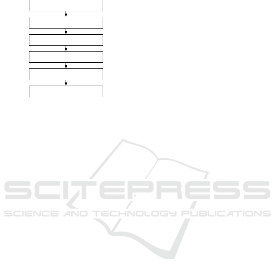
Generation of the complex data set
Data basis
Stochastic modelling
Separation in microtrips
Combinatorics
RDE speed curve
Figure 2: Schedule for generating replacement cycles.
plification by means of a so-called Markov assump-
tion (memorylessness). Due to this, a system’s sub-
sequent state is only dependent on the current state,
which causes preceding states to have no effect at all
on the modification of states. This correlation is ex-
pressed in equation 1. x
n
represents the current state
and x
n+1
represents the subsequent one. Preceding
states as well as their impact (in equation x
1
,x
2
) are
neglected (Ließner et al., 2017). For further infor-
mation on the functionality of Markov models, see
(Stroock, 2013).
P(X
n+1
= x
n+1
|X
1
= x
1
,X
2
= x
2
,..., X
n
= x
n
) =
P(X
n+1
= x
n+1
|X
n
= x
n
)
(1)
Where,
P() = probability function,
X
n
= Markov variable,
x
n
= current state,
X
n+1
= Markov variable,
x
n+1
= following state
A state x
n
in this proposed application contains a
discrete value of velocity and acceleration as seen in
equation 2.
x
k
=
(
v
k
a
k
(2)
Where,
x
k
= state,
v
k
= velocity value,
a
k
= acceleration value
In order to transfer the data basis to the Markov
model, it is sufficient to perform an elementary iter-
ative transfer of the respective state transitions from
one point of time to the next. Further processing is
based on the assumption that the saved state transi-
tions in the Markov model hold all relevant informa-
tion concerning this relation. This is because, after all,
the Markovmodel contains all recorded drive data in a
condensed and anonymized form. However, choosing
and combining appropriate elements of the complex
data set in such a way as to allow the derivationof rep-
resentative replacement cycles with similar properties
regarding the consumption is the actual challenge.
2.3 Generation Complex Data Set
The following strategy is suitable for deriving re-
cently mixed velocity progressions from the Markov
model. Based on a velocity and acceleration combi-
nation which has been set initially, a generation can
be performed by means of a query concerning the
saved state transition according to the Markov model.
Using a weighted draw in proportion to probabilities,
the subsequent velocity and acceleration combination
is chosen. The described procedure is repeated un-
til the desired scope of the complex data set has been
attained. In this manner, an arbitrarily large data set
is generated which contains recently mixed stochas-
tically weighted progressions. But afterwards, iden-
tifying the elements in the complex data set which
ultimately best represent RDE worst case scenarios
during the substitute cycle is very challenging. To
put this into practice, it is expedient to separate the
complex data set into smaller units, which can then
be processed separately.
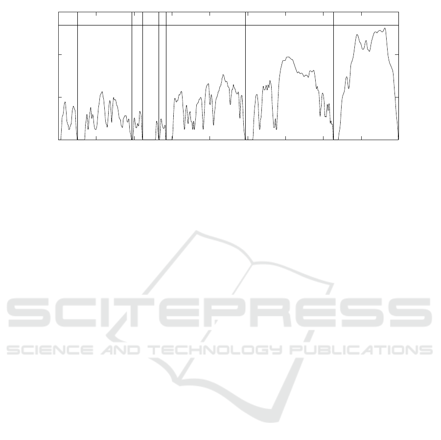
2.4 Separation Into Microtrips
For disassembling the complex date set, a fragmenta-
tion into so-called ’microtrips’ has proven to be use-
ful. A microtrip is defined as a drive starting at one
vehicle stop and finishing at the next (Fotouhi and
Montazeri-Gh, 2013). Figure 3 depicts a microtrip
segmentation into eight sections by using the WLTC
as an example. When such a segmentation is applied
to the complex data set, a very high number of mi-
crotrips is created. Finally, the major difficulty can
be seen in choosing and combining appropriate parts.
Approaches such as Lee pursue the aim of creating
vehicle-specific substitute cycles by analyzing the en-
ergy level at the periphery of the wheels and then
producing a selection of statistical key figures (Lee
and Filipi, 2010). In contrast to this, this contribu-
tion aims for a vehicle-independent combinatorics at
first. This combinatorics would contain properties oc-
curring during the substitute cycle which are relevant
for driving dynamics: distribution (velocity, accelera-
tion, velocity multiplied by acceleration and stop) and
VEHITS 2017 - 3rd International Conference on Vehicle Technology and Intelligent Transport Systems
190
0 200 400 600 800 1000 1200 1400 1600
time in s
0
50
100
150
velocity in km/h
1 2 3 4 5 6 7 8
Figure 3: Separation of a drive in microtrips at the example of the WLTC.
the relative positive acceleration (RPA) index. Single
microtrips have to be combined into one single sub-
stitute cycle in order to have high dynamic RDE con-
formable cycle as closely as possible. To achieve this,
the following procedure can be employed.
2.5 Combinatorics
The main challenge in generating RDE substitute cy-
cles is combining the previously created microtrips in
such a manner as to form a substitute cycle, which
will then conform to the relevant RDE criteria.
Theoretically, it would be possible to try out all
variants (brute force method). Yet it becomes clear
that in a complex data set with K microtrips and for
the replacement cycle E necessary ones, K
E
combi-
nations emerge. For example, K = 1000 available
and ordinary E = 20 for the RDE replacement cy-
cle necessary microtrips as well as the assumption
that an evaluation takes 0.1 seconds, a duration of
2.7· 10
15
hours for the generation of the replacement
cycle would be set. Thus a brute force approach for
combination is not suitable (Ließner et al., 2017).
The RDE combinatorics outlined here is based on
the combinatorics for generating average substitute
cycles, as presented in (Ließner et al., 2017). In the
mentioned paper, a method is presented which en-
ables the combination of microtrips to form a sub-
stitute cycle by employing a so-called Threshold Ac-
cepting combinatorics algorithm. This procedure en-
sures that vehicle dynamic will be maximized.
Using an average substitute cycle as a basis for
RDE combinatorics has multiple advantages. RDE
certification has the fundamental aim of defining
boundary conditionswhich conform as closely as pos-
sible to real driving situations. Thus, it is made pos-
sible that an average cycle, which must feature the
respective duration and driving mode share, nearly or
completely meets RDE standards from the beginning
on. The following methodology uses the average sub-
stitute cycle and modifies included shares until all cri-
teria are met. The modification is performed in ac-
cordance with the Threshold Accepting Method first
introduced in (Ließner et al., 2017). This is an algo-
rithm presented by Prof. Dueck to solve combinato-
rial problems (Dueck and Scheuer, 1990).
Besides meeting RDE standards, one additional
aim is to maximize vehicle dynamics. According
to RDE guidelines, the vehicle dynamics limit is as-
sessed by determining va
pos
_95 values for the respec-
tive area (urban, rural, motorway). These values rep-
resent, in dependence of average velocities, threshold
values ¯v
k
which must not be exceeded. The following
equation illustrates the exemplary conditions for the
urban area.
(v· a
pos
)
urban,ref
_95 ≤ (0.136· ¯v
urban
+ 14.44) (3)
Where,
(v· a
pos
)
urban,ref
_95 = 95th percentile va
pos
value,
¯v
urban
= average urban speed
The respective intermediate steps and the algo-
rithm for calculating va
pos
_95 can be found in (Eu-
ropean Commission, 2016). Hence, minimizing the
difference between the actual va
pos
_95 values and re-
spective set values can be seen as a possible approach
for the maximization of vehicle dynamics. The fol-
lowing function is a measure of quality for optimising
va
pos
_95 values:
J =
∑
k
w
k
·((v·a
pos
)
k,ref
_95−(v·a
pos
)
k,cur
_95)) (4)
Where,
k = {urban, rural, motorway},
(v· a
pos
)
k,ref
_95 = set value of 95th percentile,
(v· a
pos
)
k,cur
_95 = actual value of 95th percentile,
w
k
= number of elements with a
k
> 0.1m/s
2
Derivation of Real Driving Emission Cycles based on Real-world Driving Data - Using Markov Models and Threshold Accepting
191

The sampling of all courses, which have been used
in the context of RDE, is generally 1 Hz. Since the
route that is to be completed has the same length
of at least 16 km in all speed ranges, it can be de-
rived that the urban area exhibits the largest number
of measured values and hence, also the largest num-
ber of va
pos
_95 values. This consideration helps to
determine the weighting (equation 4). In this man-
ner, it can be ensured that the optimization preferably
covers the urban speed range. The weighting corre-
sponds logically to emission layers as well, since fre-
quently occurring partial loads, engine operation in
the scavenging range and unfavourable regeneration
conditions cause increased emissions in urban areas.
The va
pos
_95 value is only one scalar that characterise
the vehicle dynamicof the whole RDE cycle. It can be
used to check the validity of a RDE cycle. If it is the
aim to get the maximum possible vehicle dynamic in
a cycle all the sampling points around va
pos
_95 need
a high dynamic too. In the RDE context it means
that all sampling points under the va
pos
_95 bound-
ary, which is equivalent to 95 % of the elements with
a
k
> 0.1 in the respective area, should attain va
pos
val-
ues as close as possible to the va
pos
_95 value. The
other sampling points (5 %) should achieve the maxi-
mum possible dynamic of the respective vehicle.
Algorithm 1: RDE replacement cycle generation.
1: Load average cycle
2: Choose initial THRESHOLD T > 0
3: As long as improvement occurs
4: Modify driving cycle slightly (change one microtrip)
5: Calc. ∆E := quality(old conf.)-quality(new conf.)
6: If ∆E > T & RDE-criteria are satisfied
7: THEN old conf. := new conf.
8: If for too many iterations no improvement
9: THEN lower THRESHOLD T
10: If no further improvements are made
11: THEN stop
12: End
calc. = calculate, config. = configuration
As can be understood through pseudocode above,
the combination process begins with an average sub-
stitute cycle featuring a length of 6300 seconds ±14
% (line 1) which met the RDE trip duration between
90 and 120 minutes. Additionally, an initial thresh-
old value T > 0 controlling the optimization process
has been set for the optimization (line 2). In (Dueck
and Scheuer, 1990), Prof. Dueck indicates that the
threshold parameter does not react very sensitively
to the solution quality and hence, does not have to
be elaborately optimized. Consequently, the iterative
modification of the initially assembled substitute cy-
cle commences (line 3-12). During each respective
loop run, the substitute cycle is slightly modified (line
4). This modification is achieved by randomly chang-
ing one of the E microtrips. Instead, a microtrip in
the complex data set is randomly chosen and then put
in. A subsequent evaluation of the quality assesses
this modification. The modified substitute cycle is
only adapted as a new reference, if the quality has
improved for more than the given threshold value T,
if the resulting cycle meets all RDE standards and
the resulting cycle length corresponds to the prede-
fined interval (line 5-7). By means of two further in-
ner loops, an adaptation of the optimization process
is achieved. On the one hand, the threshold value T
is reduced after a certain number of inexpedient mod-
ifications (line 8-9), which incrementally reduces the
subsequent cycle’s demanded improvement as well.
These consequences lead to the fact that only solu-
tions performing substantially better can be adapted
as a new reference solution. The demanded improve-
ment is mitigated by the reduction of threshold val-
ues during the optimization process. But on the other
hand, the optimization process will be terminated if
after a large number of modifications, no further im-
provement has been achieved (line 10-11). This prac-
tice ensures that the optimization is only performed
in correspondence to the achievement of improve-
ments. Taking sample solutions during the optimiza-
tion process is made possible by the iterative approach
(Ließner et al., 2017).
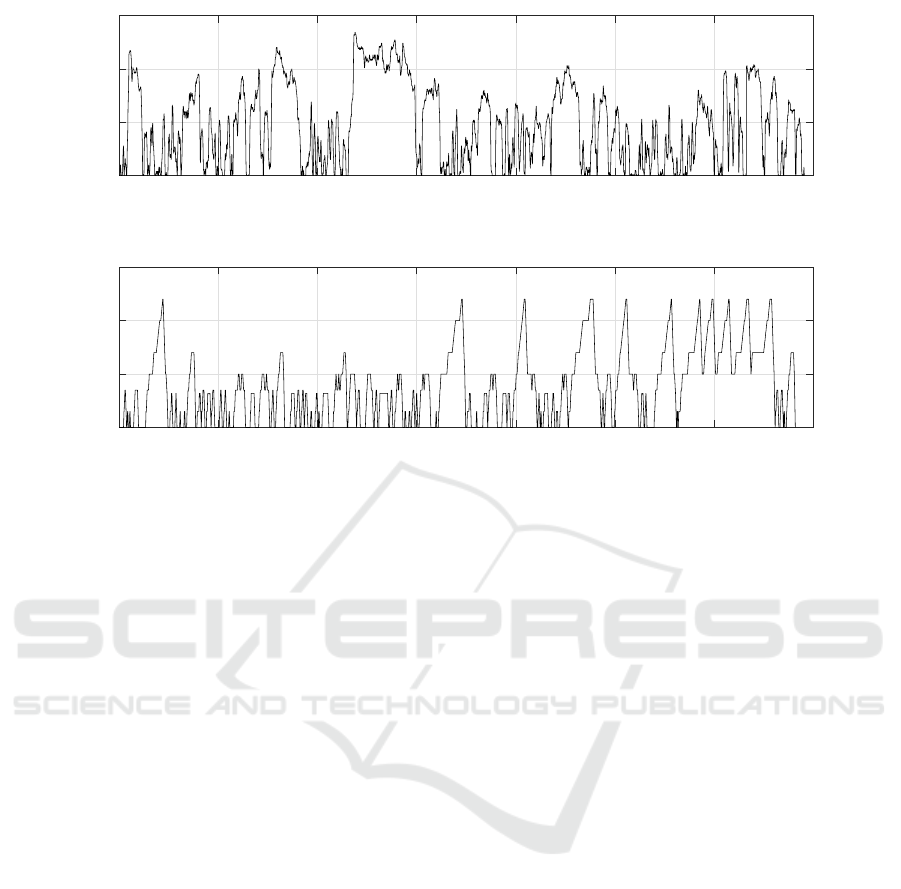
3 RESULTS
This chapter illustrates various results of the gener-
ation of RDE replacement cycles which will be dis-
cussed in the following subsections. For the presen-
tation of individual aspects two examples based on
different data sets were prepared. The velocity curves
are shown in Figure 4 and 5. Figure 4 represents real
driving data. The cycle in Figure 5 was generated
with NEDC velocity curves. With the help of the re-
placement cycle based on the NEDC data it can be
demonstrated very well that the presented algorithm
provide the desired results. The evaluation of the cy-
cles from Figure 4 and 5 concerning to the RDE cri-
teria is shown in Table 1. It compares the different
characteristic values of the replacement cycles with
the given values of the RDE legislation.
3.1 Fulfillment of the RDE
Requirements
As is demonstrated in Table 1, all RDE standards con-
cerning vehicle dynamics can be met. This is not only
VEHITS 2017 - 3rd International Conference on Vehicle Technology and Intelligent Transport Systems
192
0 1000 2000 3000 4000 5000 6000 7000
time in s
0
50
100
150
velocity in km/h
Figure 4: RDE replacement cycle based on real driving data.
0 1000 2000 3000 4000 5000 6000 7000
time in s
0
50
100
150
velocity in km/h
Figure 5: RDE replacement cycle based on NEDC data.
the case when applying the described cycle, but by us-
ing the outlined combinatorics, any desired number of
RDE conforming cycles can be generated. The vari-
ability of usage cases is a great advantage because it
presents a broad basis for the optimization and vali-
dation of RDE cycles.
3.2 Impact of the Data Basis
The requirement for a successful generation is a rele-
vant database. Within the database, all areas (urban,
rural, motorway) have to be included to a sufficient
extent. When attempting to create a RDE cycle by us-
ing data sets which omits velocities above 90 km/h,
this demand becomes much more transparent. In the
case stated above, the missing velocity shares render
a successful combinatorics impossible.
The respective route areas (urban, rural, motor-
way) are automatically determined by the employed
combinatorics. The specific distribution is not af-
fected in any way. The fundamental area distribu-
tion is shaped by the database’s quality. In this con-
text, the adherence to the permitted maximum veloc-
ity is not problematic. By screening microtrips with
higher maximum velocities than 160 km/h out of the
database beforehand, an expedient violation of this
criterion can occur.
3.3 Distribution of Stoppages
Stoppages (v = 0) within the original data have a sig-
nificant role for an expedient combinatorics. The cy-
cle parameters ’average v
urban
’, ’stop ratio urban’, as
well as ’stops above 10 s’ and ’stops above 180 s’ un-
derline this. These parameters will not be represented
correctly in the substitute cycle if the stoppages do not
have the relevant quality.
In contrast to selecting suitable shares with a ve-
locity higher than zero, the generation of stoppages
(v = 0) is much more simple. Since these stoppages
only incorporate sequences of velocities of the value
zero, additional editing is possible. If, for example,
the criterion ’stop share urban’ > 10% has not been
met, the criterion can be fulfilled by manipulating the
already existing stoppages during the post processing.
However, the longest permitted driving duration must
not be violated.
The calculation of the va
pos
_95 and RPA values
only consists of measurements with a acceleration of
a > 0.1m/s
2
. Nonetheless, the assessment for validat-
ing vehicle dynamics is based on the average veloci-
ties of each area. Regarding the urban area, stoppages
are incorporated into the calculation as well.
3.4 Analysis of Replacement Cycles
The RDE substitute cycle, which is based on the
NEDC data set (see Figure 5), evidently contains a
great number of linear acceleration courses, such as
can also be found in the NEDC. The maximum ac-
celeration values are comparable to those found in the
NEDC. This attribute is also very prominent in the
NEDC and leads to the use of only a few engine op-
eration points while driving the cycle. The cycle in
Derivation of Real Driving Emission Cycles based on Real-world Driving Data - Using Markov Models and Threshold Accepting
193

Table 1: Fullfillment of RDE requirements of the generated cycles.
Requirement Unit Set Value RDE Cycle NEDC RDE Cycle Real Driving
Trip duration [min] 90-120 113.63 105.40
Urban operation [%] 29-44 43.92 32.16
Rural operation [%] 23-43 26.43 30.82
Motorway operation [%] 23-43 29.65 37.01
Urban distance [km] ≥ 16 32.00 26.20
Rural distance [km] ≥ 16 19.25 25.11
Motorway distance [km] ≥ 16 21.60 30.15
Maximum speed [km/h] 145 120 134
Time v > 100 km/h [min] ≥ 5 6.65 10.82
Average Speed urban [km/h] 15-40 km/h 22.44 23.03
Stop ratio urban [%] ≥ 10 28.44 13.06
Stop t > 10 s [#] ≥ 2 51 16
va
pos
_95 urban [m
2
/s
3
] < 17.57 7.72 16.05
va
pos
_95 rural [m
2
/s
3
] < 24.51 10.03 24.23
va
pos
_95 motorway [m
2
/s
3
] < 26.87 9.10 26.39
RPA urban [m/s
3
] > 0.14 0.14 0.28
RPA rural [m/s
3
] > 0.06 0.11 0.15
RPA motorway [m/s
3
] > 0.025 0.12 0.10
figure 5 ranks near the lower limit of the RPA value
for urban and ranks thereby also near the lower limit
of permitted vehicle dynamics. This effect highlights
how much more dynamic the drives used for the RDE
assessment will be compared to the ones that have
been used so far.
In contrast to this, the driving cycle based on real
drives (see Figure 4) represents a cycle ranked near
the higher limit for driving dynamics. A specific max-
imum value for the va
pos
_95 values cannot be derived
more easily, because the relevant reference value is
calculated by using the average velocity. The dis-
cussed phenomena concerning the NEDC substitute
cycle do not occur in this cycle, which is much more
similar to a real drive when looking at the character-
istics.
3.5 Worst Case Scenario
The worst-case cycle in connection to RDE driving
cycles has already been a subject of discussion in the
beginning of this paper. What is meant in this case
is a set of driving cycles, which operate the assessed
vehicle near the RDE validity limit. The objective has
to be that passing the RDE assessment by using these
cycles must ensure that all possible drives conform-
ing to RDE will pass the assessment. It has already
been discussed in section 2.1 that the paper at hand
only gives a first, partial solution. Nevertheless, the
emissions have to be maximized already during this
partial step. One approach would be to increase the
driving cycle’s dynamics, which would also increase
the emissions regarding vehicles with a combustion
engine.
Another determining factor for the increase of
emissions during a driving cycle is the distribution of
stoppages (v = 0). Especially the conditions in the
exhaust gas aftertreatment system play an important
role here. To give an example, it is well-known that a
certain temperature in catalytic converters is a prereq-
uisite for best executing the required reaction of re-
ducing emissions. Should this not be the case, signif-
icantly higher values will occur during the cold start
phase. Even extensive idle times during a drive can
lead to similar effects. Such pauses should be imple-
mented into the worst-case case in a manner which
enables cooling processes to repeatedly cause compa-
rable situations.
A worst case cycle should also contain high dy-
namic maneuvers in the cold start phase. The end of
that cold start phase is defined by a temperature of the
coolant over70
◦
C or after fiveminutes in the wording
of the law. So most of the combustion engines espe-
cially in cold environments don’t reach their normal
operating temperature during this time.
4 SUMMARY AND OUTLOOK
In the contribution at hand, the possibility of generat-
ing RDE cycles from real driving data has been il-
lustrated. By applying the outlined approach, spe-
cific substitute cycles for different types of vehicles
VEHITS 2017 - 3rd International Conference on Vehicle Technology and Intelligent Transport Systems
194

or markets, which can differentiate greatly in char-
acteristics or velocity distribution, can be developed.
The possibility of generating a large quantity of dif-
ferent cycles and using them during the development
process makes the avoidance of phenomena such as
cycle beating possible.
The main focus was not only on the generation of
RDE cycles, but these cycles were also supposed to
cause a larger quantity of emissions in the assessed
vehicles. To meet the requirements in a first step,
the maximum permitted dynamics in the contest of
RDE ambient conditions were demanded. Addition-
ally, considerations were presented which increase
emissions due to the chosen sequence of operational
conditions, regardless of strictly set requirements.
In the future, RDE cycles will play an important
role in both the vehicle development and the assess-
ment of vehicle emission values. At present, RDE
drives are commonly selected on the basis of impre-
cise compilations of driving road criteria (see Table 1)
and then traced on real roads. This procedure is on the
one hand very time-consuming, and on the other hand
does not guarantee that RDE requirements will be
met, especially when unpredictable disruptions such
as traffic jams occur. At some point, the recording
of RDE measurement drives will predominantly take
place on chassis dynamometers, since these can be
adapted to be nearly identical to the chosen ambient
conditions and can also follow the set velocity course
precisely.
During vehicle development, the usage of simula-
tions and procedures such as the model-based calibra-
tion will gain more importance due to RDE require-
ments. Even now, engineers face the challenge of
constantly reducing development periods and steadily
increasing numbers of vehicle variants while still us-
ing conventional development methods. Thus, the
majority of calibration will be executed at the com-
puter and at test benches of different complexity. A
significant part of this practice will be various driv-
ing cycles, because they constitute the most realistic
testing scenarios in vehicle development.
Further contributions can continue the gradual
generation of RDE worst-case cycles (see Section
2.1). Correspondingly, an elevation profile will be
overlaid in a next step, after which vehicle-specific
cycles can be derived. Based on this procedure, one
obtains a set of cycles representing the worst-case
case concerning emissions for the respective vehicle.
REFERENCES
Dueck, G. and Scheuer, T. (1990). Threshold accepting:
A general purpose optimization algorithm appearing
auperior to simulated annealing. Journal of Computa-
tional Physics, 90(1):161–175.
European Commission (2016). Comission Regulation (EU)
2016/646. Official Journal of the European Union.
Fotouhi, A. and Montazeri-Gh, M. (2013). Tehran driv-
ing cycle development using the -means clustering
method. Scientia Iranica, 20(2):286–293.
Fraidl, G., Kapus, P., and Vidmar, K. (2016). The gaso-
line engine and RDE challenges and prospects. In 16.
Internationales Stuttgarter Symposium, Wiesbaden.
Springer Fachmedien.
Gerstenberg, J., Hartlief, H., and Tafel, S. (2016). Introduc-
ing a method to evaluate RDE demands at the engine
test bench. In 16. Internationales Stuttgarter Sympo-
sium, Wiesbaden. Springer Fachmedien.
Lee, T.-K. and Filipi, Z. S. (2010). Synthesis and validation
of representative real-world driving cycles for plug-
in hybrid vehicles. In 2010 IEEE Vehicle Power and
Propulsion Conference (VPPC), pages 1–6.
Ließner, R., Dietermann, A., Lüpkes, K., and Bäker, B.
(2017). Generation of replacement vehicle speed cy-
cles based on extensive customer data by means of
markov models and threshold accepting. SIAT - Sym-
posium on International Automotive Technology 2017.
Maschmeyer, H., Beidl, C., Düser, T., and Schick, B.
(2016). Real Driving Emissions - Ein Paradigmen-
wechsel in der Entwicklung. MTZ - Motortechnische
Zeitschrift, 76:36–41.
Steinbach, M., Neumann, T., Kutzner, A., Lehmann, V.,
Kassem, V., and Dreiser, M. (2016). Model sup-
ported calibration process for future RDE require-
ments. In 16. Internationales Stuttgarter Symposium,
Wiesbaden. Springer Fachmedien.
Stroock, D. W. (2013). An introduction to Markov pro-
cesses. Graduate texts in mathematics. Springer,
Berlin, 2nd edition.
Derivation of Real Driving Emission Cycles based on Real-world Driving Data - Using Markov Models and Threshold Accepting
195
