Exploring Text Classification Configurations
A Bottom-up Approach to Customize Text Classifiers based on the Visualization of
Performance
Alejandro Gabriel Villanueva Zacarias, Laura Kassner and Bernhard Mitschang
Graduate School of Excellence Advanced Manufacturing Engineering, Nobelstraße 12, 70569 Stuttgart, Germany
Keywords:
Data Analytics, Unstructured Data, Text Data, Classification Algorithms, Text Classification.
Abstract:
Automated Text Classification (ATC) is an important technique to support industry expert workers, e.g. in
product quality assessment based on part failure reports. In order to be useful, ATC classifiers must entail
reasonable costs for a certain accuracy level and processing time. However, there is little clarity on how
to customize the composing elements of a classifier for this purpose. In this paper we highlight the need
to configure an ATC classifier considering the properties of the algorithm and the dataset at hand. In this
context, we develop three contributions: (1) the notion of ATC Configuration to arrange the relevant design
choices to build an ATC classifier, (2) a Feature Selection technique named Smart Feature Selection, and (3) a
visualization technique, called ATCC Performance Cube, to translate the technical configuration aspects into
a performance visualization. With the help of this Cube, business decision-makers can easily understand the
performance and cost variability that different ATC Configurations have in their specific application scenarios.
1 INTRODUCTION
As companies generate more detailed data about their
processes, the complexity to manage and improve
them increases as well. Also, market demands con-
tinuously challenge them to analyze more than just
structured data. This is relevant because unstructured
data, mostly text, accounts for at least 80% of all cor-
porate data (Ng et al., 2013). Hence the potential
to effectively integrate and analyze unstructured text
data to do better decision-making, insightful planning
and flexible processes (Kemper et al., 2013).
To succeed, there are two sources of complexity to
master: 1) data heterogeneous formats, contents and
sheer size, and 2) the many possible ways to apply
data analytics methods. If companies do not address
issues derived from them, they can overspend strate-
gic resources trying to develop appropriate analytics
solutions without satisfactory results. Thus a central
question is: how can decision-makers ensure the so-
lutions they invest in truly meet their needs?
Automated Text Classification (ATC) is one such
case. By making use of previously categorized docu-
ments and appropriate Machine Learning techniques,
ATC classifiers can efficiently sort out new documents
into the considered categories (Sebastiani, 2002). For
example, (Kassner and Mitschang, 2016) describe an
application scenario where workers have to catego-
rize messy data: short free-text reports with abundant
abbreviations, technical and organizational terms, and
spelling mistakes.
In this paper we discuss ways in which ATC
classifiers can be configured and how seemingly
small differences can bring considerable performance
changes. In section 2 we describe the dataset and
the underlying industrial business process used in this
work. In section 3, we introduce ATC Configurations
(ATCCs). With them, we can go through the differ-
ent design aspects involved in building ATC classi-
fiers under the Vector Space Model. We also intro-
duce here a Feature Selection technique that greatly
improves efficiency. In Section 4 we describe the im-
plementation of 40 ATCCs to demonstrate the perfor-
mance variability and malleability of ATC classifiers.
In section 5 we present the ATCC Performance
Cube. This visualization enables business decision-
makers to compare and select, among many, the most
suitable ATCC for a particular scenario. With this tool
decision-makers can grasp the effect of technical de-
sign choices and the potential trade-offs to be made.
We point to similar works as comparative refer-
ence in Section 6 and conclude in Section 7 by re-
flecting on the reach and further development of our
contributions.
504
Zacarias, A., Kassner, L. and Mitschang, B.
Exploring Text Classification Configurations - A Bottom-up Approach to Customize Text Classifiers based on the Visualization of Performance.
DOI: 10.5220/0006309705040511
In Proceedings of the 19th International Conference on Enterprise Information Systems (ICEIS 2017) - Volume 1, pages 504-511
ISBN: 978-989-758-247-9
Copyright © 2017 by SCITEPRESS – Science and Technology Publications, Lda. All rights reserved

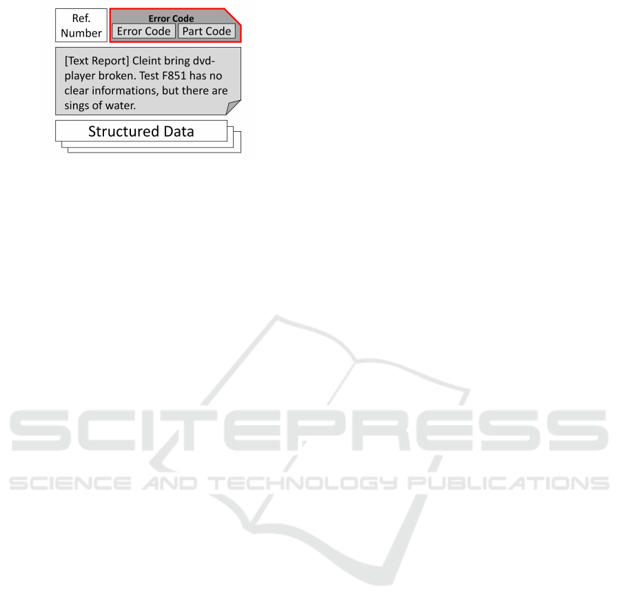
Figure 1: Selected data bundle in our application scenario.
2 DATASET AND APPLICATION
SCENARIO
2.1 The Dataset
Our study dataset refers to an after-sales quality man-
agement process in an automotive company. It con-
sists of unstructured text reports written by workers
of a supplier company in either English or German.
It comprises 7500 cases of failed car parts analyses.
Figure 1 shows the structure of what we call a data
bundle, consisting of a single text report and its com-
plementary data. Each bundle deals with a single part
and is identified with a unique reference number.
Knowledge workers assign error codes (made of
part type + failure type) to the reports. These are the
different classification categories we are interested in.
The main content of our bundle is a free-text re-
port. Containing only 33 terms on average, its con-
tents can be characterized as messy data (Kassner
and Mitschang, 2016) due to spelling errors, abundant
domain-specific abbreviations and terminology.
Along with the text reports, we also consider some
structured data metrics describing the state of the car
containing the part, such as: the distance driven be-
fore the failure and the date when the car was initially
registered. Since our focus remains on text mining
and ATC, we consider these data a secondary source.
2.2 The Application Scenario
With 1271 different error codes in this dataset, our
classification problem can be considered a highly mul-
ticlass (Gupta et al., 2014) one. It entails high com-
plexity to correctly assign documents to a category
and can thus become very time-consuming if per-
formed solely by humans. A better way to handle this
is to have an ATC classifier suggesting error codes to
knowledge workers.
Due to this purpose, we select two types of per-
formance metrics: (1) classification accuracy (includ-
ing the right error code in the list of suggestions) and
(2) the time per report (how long it takes to classify
a single report). We consider accuracy at two cut-off
levels (1 and 5). For time, we measure the classifica-
tion time per report from a testing set. Choosing these
metrics also allow us to do a direct comparison with
the results of (Kassner and Mitschang, 2016).
From a business perspective, these metrics are rel-
evant because (1) more accurate suggestions mean
more value generated by the ATC classifier; (2) the
less time it takes to classify a report, the less comput-
ing time is needed, meaning lower costs and better use
of resources. Also, different business priorities can
determine desirable performance trade-offs between
these metrics to suit a certain application scenario.
So if a company wants to reply with custom auto-
mated responses to customer support requests based
on the customer’s language, the described problems,
etc. (the customer support scenario), speed may be
more valuable than accuracy. Similarly, if misclas-
sified customer complaints lead to higher reimburse-
ments (the complaint reimbursement scenario), as-
signing the wrong category becomes a bigger concern
than taking extra time to do the classification.
3 DESIGN ASPECTS OF AN ATC
CLASSIFIER
Any ATC classifier requires transforming text doc-
uments into a representation that can be analyzed.
One way to do this is under the Vector Space Model
(VSM) by (Salton et al., 1975). In it, every docu-
ment is turned into a vector with all distinct terms in
the dataset (usually distinct single words) being rep-
resented by their frequencies. In this way, each term
can be used as a feature to analyze documents.
The specifics to use this model are determined by
choices made on many design aspects as discussed by
(Hotho et al., 2005), (Dasgupta et al., 2007) and (Se-
bastiani, 2002). They usually belong to one of two
groups: (1) those to transform documents into vec-
tors, and (2) those that build the classifier’s logic using
this vectorial representation. Examples are: data rep-
resentation, term frequency schemes, pre-processing
methods, feature selection techniques, dataset split-
ting and sampling, etc.
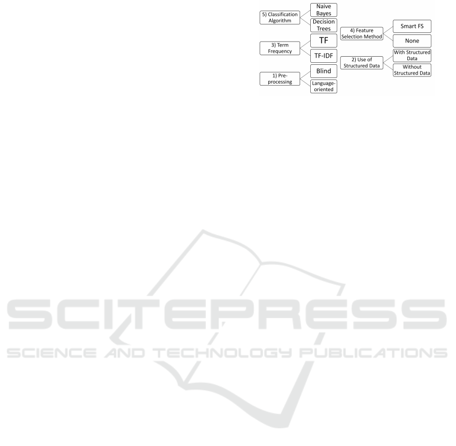
In our case, we divide them into three groups in-
stead (see Figure 2): (1) aspects to generate the fea-
tures to train the classifier, (2) aspects to the reduce
the resulting feature set and make the classifier more
efficient, and (3) aspects related to the algorithm used.
Exploring Text Classification Configurations - A Bottom-up Approach to Customize Text Classifiers based on the Visualization of
Performance
505

Figure 2: Design aspects to consider in our Automated
Text Classification Configurations and their corresponding
choices.
Each group becomes a layer of what we define as an
ATC Configuration (ATCC), a coherent set of valid
design choices in each of the three layers that result
into an ATC classifier. Choices on each layer should
be compatible with each other to produce a functional
ATC classifier. Therefore, choosing to remove num-
bers from a concept-based feature set would not be
part of a valid ATCC.
ATCCs evidence (1) that building a classifier can
be seen as a bottom-up process: starting with the
dataset properties and making choices to find a suit-
able algorithm, (2) that algorithms are just one of
many classifier components, (3) what exactly differ-
entiates classifiers, easing exploration and compari-
son. The following subsections detail each layer for
our application scenario.
3.1 Feature Generation Aspects
We consider up to four ways to transform the
dataset text reports into feature vectors, namely (1)
with different data representations, (2) applying pre-
processing filters (stop word removal, lowercasing,
etc.), (3) with different term frequency schemes, and
(4) adding structured data features.
3.1.1 Data Representation
We select two well-established base representations:
Bag of Words (BoW), where every word in text
becomes a classification feature and Bag of Con-
cepts (BoC), where only words or word combina-
tions recognized as labels of a domain-specific con-
cept are considered classification features. We re-
place each concept mention with a concept ID from
a domain-specific taxonomy as done by (Kassner and
Mitschang, 2016).
3.1.2 Pre-processing
On top of the BoW representation, we apply two
kinds of pre-processing that we call language-blind
Table 1: Text Reports Datasets.
BoW Language
blind
BoW Language
oriented
BoC
Train Split 4,811 3,768 4,555
Test Split 1,482 1,230 2,157
Total Documents 6,293 4,998 6,712
Total Terms 8,219 9,307 852
and language-oriented
1
. In the first case, we apply
lowercasing, remove stop words from both English
and German (thus being blind to the document’s lan-
guage), remove numeric digits and punctuation signs.
Language-oriented pre-processing does the same
steps plus language recognition before stop word re-
moval (to target only the identified language), and
stemming as a final step. Due to the data messi-
ness, language recognition cannot identify some re-
ports as English or German, which results in the re-
port being discarded. This explains why the BoW
language-oriented dataset has considerably less doc-
uments than BoW language-blind (6293 versus 4998)
(third row on Table 1). However the fourth row shows
language-oriented pre-processing also produces more
terms, thanks to not removing terms falsely identified
as stop words from the other language. Subsequent
steps (sampling, classifying) with this pre-processing
are performed keeping the language ratios.
The rest of the design aspects do not alter the total
number of documents considered in any dataset.
3.1.3 Term Frequency
We calculate each feature’s weight (term or concept)
in two manners: Either using the frequency count in
the report it is contained (term frequency), or with the
tf-idf scheme (term frequency - inverse document fre-
quency).
3.1.4 Use of Structured Data Features
We either include structured data metrics as features
(the date when the car was initially registered and the
time it spent on the road) or we use the BoW and BoC
datasets alone. These metrics were selected from the
ones available in the data bundle based on the variabil-
ity they could contribute to differentiate classification
categories.
3.2 Feature Selection Aspects
Feature Selection techniques increase the efficiency
of an ATC classifier by reducing the number of fea-
tures to use. In our study, we have a single design
choice only for the BoW datasets (given the small
1
BoC representations are not subject to pre-processing.
ICEIS 2017 - 19th International Conference on Enterprise Information Systems
506

1000 terms after the top
20% most frequent terms
Features (terms) ordered by frequency
Figure 3: Subset logic of the Smart Feature Selection tech-
nique.
number of features in the BoC dataset). We either
use a new technique called Smart Feature Selection
(Smart FS) or employ all features. This technique
is based on the properties of power-law distributions
typically found in word frequency (Newman, 2005).
To assume the existence of this distribution in our
data we use the Kolmogorov-Smirnov (KS) statistic
and the p-value from a hypothesis test as proposed by
(Clauset et al., 2009). The former estimates the differ-
ence between a fitted power-law distribution and the
actual data, while the latter tests if the data does not
come from a power-law distribution. Near zero val-
ues of the KS statistic and a p-value above 0.05 can
validate our power-law distribution assumption. Cal-
culations on the dataset most closely resembling the
original data
2
yield a KS statistic of 0.006783 and a
p-value of 0.051216, thus satisfying the requirement.
We can then assume feature rankings in our
datasets to resemble that in Figure 3. As we move
to the right side of this graphic we find the potential
useless features (Liu et al., 2013), which are so rare
to be common even in the category of the documents
they belong to. The less frequent they are, the less
useful they are to classify documents. On the left side
we see the very frequent features. The more frequent
they are, the more we can expect them to be present
across multiple categories. This is specially true for
highly multiclass problems like ours. It is clear that a
middle selection of relatively frequent features is the
most appropriate in our scenario.
Therefore, our Smart Feature Selection technique
1) discards very frequent features accounting for at
least 20% of the term instances (or tokens) in a
dataset, 2) selects the following 1000 features, and
3) discards the remaining nearly useless ones. In
the case of the language-oriented dataset, we apply
this technique maintaining the language ratios. This
means 58% of the selected features are obtained from
English, while the remaining 42% are German.
2
with unchanged frequency values, namely the BoW -
blind pre-processing -TF weights
Table 2: Smart Feature Selection values on datasets.
Share of all
distinct terms
Share of all to-
kens in dataset
Total terms
in dataset
BoW-Blind
dataset
12.17% 70.64% 8219
BoW-Language-
oriented dataset
10.74% 63.05% 9307
Using Smart Feature Selection implies the claim
that a relatively small number of features with the
right frequency can provide good enough coverage of
our datasets, which in essence is an adaptation of the
80/20 heuristic focusing on the significant few. Table
2 shows the resulting coverage ratios on the applica-
ble datasets (those with BoW representations, see Ta-
ble 1). They validate our heuristic claim: although
1000 terms represent a small proportion of the total
number of terms (first column), they account for a
big share of the tokens (term instances) in the dataset
(second column).
Better coverage ratios may be obtained either by
augmenting the number of selected terms, or by start-
ing the selection at some other threshold. For scenar-
ios aiming to get higher accuracy (e.g. the complaint
reimbursement scenario in subsection 2.2), this can
be worthy future work.
3.3 Classification Algorithm Aspects
Based on our application scenario, we select the al-
gorithms to use with the following criteria: (1) typi-
cal text mining algorithms known for their high accu-
racy; (2) ability to handle hundreds of possible clas-
sification categories; (3) ability to integrate different
feature types, so that unstructured and structured fea-
tures can be used together.
As a result we select the Naive Bayes and Deci-
sion Trees algorithms. The first one is a probabilis-
tic algorithm that produces good results thanks to its
Naive assumption of considering the terms’ existence
and order independent from one another (Hotho et al.,
2005). Moreover, it can be effectively trained with a
small amount of data making it able to handle classi-
fication categories with few reports, as is our case.
Decision Trees are considered a very fast and scal-
able algorithm thanks to its simple logic to recursively
split train data based on one feature at a time (Hotho
et al., 2005). In our case, the classification model is
built based on the highest Information Gain.
In both cases, we generate class probabilities for
every document in the dataset to obtain a list of cate-
gory suggestions. With them we evaluate each algo-
rithm’s accuracy@1 and accuracy@5. We also mea-
sure the time to classify each document in our testing
set (Classification time per report).
Exploring Text Classification Configurations - A Bottom-up Approach to Customize Text Classifiers based on the Visualization of
Performance
507

4 ATCCs IMPLEMENTATION
With choices for every design aspect made in the pre-
vious section (summarized in Figure 4), we build 40
ATCCs. Out of them, 32 are built by combining the
choices of all five aspects for BoW datasets. The re-
maining 8 only combine the choices of the relevant
aspects for the BoC dataset (numbered 2, 3, and 5 in
Figure 4).
Having two choices per design aspect is inten-
tional. As we seek to demonstrate performance vari-
ability and the utility of arranging multiple design as-
pects into ATCCs, two choices per design aspect are
the minimum to generate combinations (2
5
+ 2
3
).
4.1 Validation Setup
We run our ATCCs in a dual-core Linux server run-
ning at 2 Ghz with 50 Gb of memory. Data is initially
retrieved from a relational database. The concept an-
notation is done using a UIMA pipeline (Ferrucci and
Lally, 2004) and a taxonomy file with the domain-
specific concepts to identify following the approach
of (Kassner and Mitschang, 2016). Further steps are
done with R scripts.
Every time we run an ATCC, we build train
and test sets using stratified simple random sampling
without replacement. We sample around 20% of all
data for the test dataset. The resulting sizes of the
train and test datasets can be seen on rows 1 and 2 of
Table 1. In all cases we make sure that every classi-
fication category has at least two documents before
splitting. This both ensures the classifier is tested
against valid documents only, and leads to the loss of
certain very infrequent classification categories (hav-
ing less than two documents).
We use standard algorithm implementations of
Naive Bayes and J48 (a Java port of the C4.5 Deci-
sion Trees’ variant) from the Weka software environ-
ment (Hall et al., 2009) in R. We also use the fol-
lowing R packages: tm (Feinerer and Hornik, 2015),
NLP, igraph (Csardi and Nepusz, 2006), SnowballC,
textcat (Hornik et al., 2013), RWeka (Hornik et al.,
2009), RPostgresql, and sampling.
Every ATCC is randomly run twice and our
selected performance metrics (accuracy@1, accu-
racy@5, and classification time per report in the test
dataset) are saved in text files.
4.2 Experimental Results
Table 3 shows a subset of results from our 40 ATCCs.
We can confirm the expected variability of using dif-
ferent ATCCs: Accuracy@1 can go from 46,30% to
Figure 4: Design aspects considered to build ATCCs and
their choices.
69,79%, while accuracy@5 varies from 59,55% to
84,22%. Overall we see that ATCCs based on the BoC
dataset have lower accuracies than their BoW counter-
parts, even if they also are considerably faster.
Also, nearly identical configurations have either
very similar or very different performance based on
the single design aspect that differentiates them. Ex-
amples of similar performance are ATCCs 1 and 3
(different by the term frequency), and 6 and 8 (with
or without SD). On the contrary, ATCCs 3 and 4 (with
a different algorithm each) have distinct Accuracy@5
and Classification Time per Report values. This sug-
gests that not all design aspects have the same effect
in performance, thus encouraging to focus on the sig-
nificant ones.
Using our Smart Feature Selection technique on
BoW configurations greatly improves Classification
Time per Report at the expense of little accuracy
losses (less than 3%). This can be seen between
ATCCs: 6 and 7, 8 and 9, 10 and 11. For config-
urations using the Naive Bayes algorithm and BoW
datasets (ATCCs 6 to 9), Smart Feature Selection re-
duces the Classification Time per Report more than 8
times with an accuracy loss of less than 2%.
Regarding differences due to the Algorithm, BoC
and BoW configurations have similar accuracy@1
values regardless of the algorithm. However at accu-
racy@5, ATCCs with Naive Bayes outperform those
with Decision Trees (dataset being equal), albeit at the
expense of longer processing times.
All in all, there is not an ATCC that outperforms
others in all aspects. Instead, ATCCs with higher Ac-
curacy tend to have longer classification times, and
vice versa. As a result, choosing an ATCC should be
done based on the trade-off that better fits the appli-
cation scenario needs.
5 ATCC PERFORMANCE CUBE
Even with a small number of configurations as pre-
sented on table 3, it is difficult to analyze differences
in performance and to recognize patterns among
ICEIS 2017 - 19th International Conference on Enterprise Information Systems
508

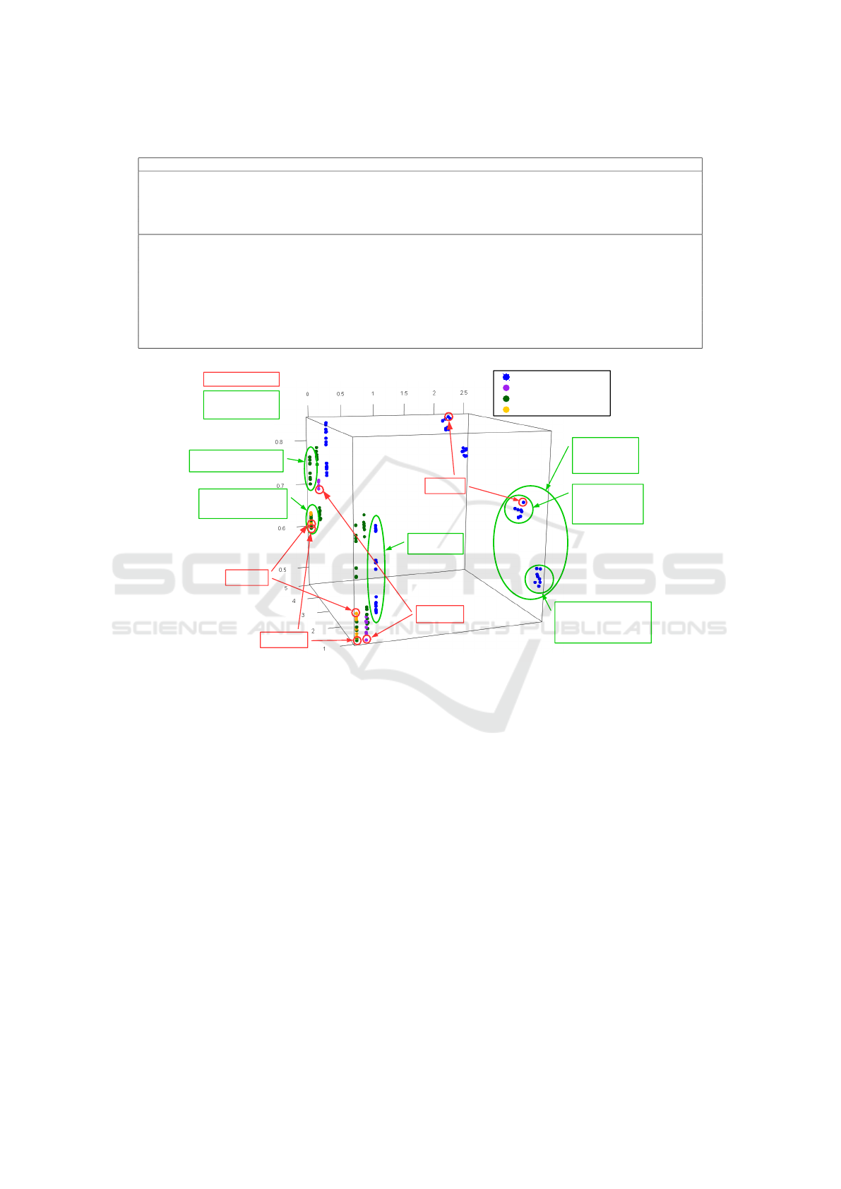
Table 3: Selected results of running 40 ATCCs. Highlighted are the best and worst values on each column.
ATCC Description Accuracy@1 Accuracy@5 Time/Report (s)
1 Concepts-Trees-TF-with SD 51,14% 61,89% 0,00169
2 Concepts-NB-TF-without SD 48,86% 70,44% 0,12908
3 Concepts-Trees-TFIDF-with SD 48,93% 60,68% 0,00167
4 Concepts-NB-TFIDF-with SD 51,00% 70,58% 0,12950
5 Concepts-NB-TFIDF-without SD 46,30% 68,80% 0,12824
6 Words-NB-Blind preprocessing-TF-with SD-Smart FS 68,64% 81,86% 0,25247
7 Words-NB-Blind preprocessing-TF-with SD-All 69,39% 81,73% 2,23463
8 Words-NB-Blind preprocessing-TF-without SD-Smart FS 67,77% 84,02% 0,25685
9 Words-NB-Blind preprocessing-TF-without SD-All 69,79% 84,22% 2,17850
10 Words-Trees-Blind preprocessing-TF-without SD-Smart FS 66,49% 75,66% 0,00395
11 Words-Trees-Blind preprocessing-TF-without SD-All 69,45% 77,55% 0,10150
12 Words-Trees-Language preprocessing-TFIDF-without SD-Smart FS 46,71% 61,66% 0,00445
13 Words-Trees-Language preprocessing-TFIDF-with SD-Smart FS 46,39% 59,55% 0,00415
14 Words-NB-Language preprocessing-TFIDF-with SD-All 55,48% 75,22% 2,51222
Full BoW
(No Smart FS)
Blind
preprocessing
Language-oriented
preprocessing
Blind preprocessing
Language-oriented
preprocessing
Time per Report (s)
Ac
c
u
ra
c
y
Cut-off
Smart FS
Naive Bayes BoW
Naive Bayes BoC
Decision Trees BoW
Decision Trees BoC
ATCC 9
ATCC 5
ATCC 13
ATCC 1
Selected ATCCs
Patterns due to
a design choice
Figure 5: ATCC Performance Cube with selected ATCCs highlighted from each data representation/algorithm combination
and identified patterns due to design choices.
them. To address this, we develop a visualization that
we call the ATC Configurations Performance Cube
(ATCC Performance Cube). It can be defined as a
three dimensional depiction of ATCCs’ performance
in terms of the selected performance metrics.
The ATCC Performance Cube with the results of
our 40 ATCCs is shown in Figure 5. The x axis shows
the classification time per report in seconds, while the
z and y axes show accuracy values at our defined cut-
off levels (accuracy@1 and accuracy@5).
The ATCC performance results serve as coordi-
nates on the corresponding axis to draw a point that
represents it. So for example, ATCC 5 from table 3
(highlighted in figure 5) can be identified as the pur-
ple point closest to the cube’s bottom cut-off 1. Mean-
while, at cut-off 5, the same ATCC can be identified
as the lowest purple point; this because other ATCCs
using Naive Bayes and BoC (e.g. ATCCs 2 and 4 from
table 3) have higher accuracies. Moreover, its classi-
fication time per report is similar to ATCCs using De-
cision Trees, BoW and no Feature Selection technique
(such as ATCC 11 from the same table) thus explain-
ing why it is aligned with them on the x axis. Other
ATCCs can be identified following the corresponding
observations.
At a glance, this visualization shows clear pat-
terns. For instance, thanks to color-coding, we can ap-
preciate the considerably lower performance of BoC
configurations compared to BoW ones. We also see
clusters of configurations in different areas of the
cube, an indicator that certain design choices have
greater effect on performance than others. The identi-
fied patterns are circled in green. We see for example
a clear divide in Time per Report among ATCCs us-
ing Naive Bayes in BoW datasets (colored in blue).
Looking them up in Table 3 (see ATCCs 6,7,8,9, and
14) we see that the design choice responsible for this
is our Smart Feature Selection technique.
Exploring Text Classification Configurations - A Bottom-up Approach to Customize Text Classifiers based on the Visualization of
Performance
509

With a similar logic we can also conclude that pre-
processing is behind the clear vertical divide among
ATCCs using BoW (like ATCCs 10 and 12 from table
3). BoC configurations do not use pre-processing and
do not show this gap, also indicating that none of their
design aspects has such an impact on accuracy.
We can also appreciate variations in accuracy due
to the algorithm as we go from accuracy@1 to ac-
curacy@5. In accuracy@1, the better performing
ATCCs of each algorithm achieve similar results (to
others with the same representation). However in ac-
curacy@5, some of the worse Naive Bayes configura-
tions are comparable to the best ones using Decision
Trees.
In summary, we can explain the agglomeration of
ATCCs in terms of Preprocessing, Algorithm and the
Feature Selection technique. This indicates that those
are the most important design aspects.
For decision-makers, the ATCC Performance
Cube reveals the trade-offs involved in switching
from one ATCC to another simply by comparing their
locations in every axis. It also allows the comparison
to an optimal performance: The closer an ATCC is to
the upper-left edge of the cube, the better it is. It is up
to the application scenario needs to determine if a se-
lected ATCC should favor classification time over ac-
curacy (e.g. the customer scenario in subsection 2.2)
or vice versa.
Using this tool, decision makers can intuitively es-
timate costs and benefits, and thus choose candidate
ATCCs that embody their priorities. Technical per-
sonnel can then select the final ATCC using the re-
maining (less) significant design choices compatible
with that selection. To realize this vision, the ATCC
Performance Cube can become a component in an ex-
ecutive dashboard in which ATCCs can be navigated,
filtered or highlighted.
The cube dimensions can be changed for other
metrics that better suit the application scenario. Re-
call or precision could be used for scenarios where
accuracy and coverage are essential. For example, for
complaint reimbursement (see subsection 2.2).
6 RELATED WORK
In this section we go over similar works to delimit the
distinctive characteristics of our contributions.
(Heimerl et al., 2012) present a visual text classi-
fier that aims to reduce the labeling effort by enabling
user-controlled classification. Their tool continuously
builds an SVM classifier for a given news dataset.
The algorithm learns to categorize documents based
on the user feedback. Although we also aim to adjust
a classifier to the dataset nature, we do not treat the
algorithm as a black box that non-experts influence.
We offer ATCCs to explore its possibilities and en-
able their comparison with cost-related performance
metrics within our ATCC Performance Cube.
(Kouznetsov and Japkowicz, 2010) propose a
method to develop classifier committees. Each can-
didate classifier is evaluated on different datasets (ti-
tles and abstracts from medical articles), its result-
ing performance metrics then projected as a multi-
dimensional vector on a two-dimensional plot. In
it, classifiers with similar performance tend to clus-
ter. Thanks to this behavior, it is possible to detect
the most competitive classifiers to build a commit-
tee. However, the vector projection and the use of
polar coordinates makes it harder for decision-makers
to determine differences among clusters. In compari-
son, our visualization depicts a metric only if needed.
Also, their approach implies that all performance met-
rics are equally relevant and understandable in every
application scenario. Still, both approaches target do-
main specific texts, aim to identify patterns visually
and depict classifiers in terms of their performance.
We also refer to the works of (Luhn, 1958) and
(Salton et al., 1975) as preceding and related ap-
proaches to our Smart Feature Selection technique.
While their concepts of word’s resolving power and
term’s discrimination value are also based on obser-
vations on statistical frequency, each one proposes a
different method to determine the most useful terms
subset. Also, there are many more approaches to im-
prove Feature Selection. Discussing them is beyond
the scope of this section. Hence we refer to the anal-
yses by (Dasgupta et al., 2007), (Naidu et al., 2014)
and (Forman, 2003) as further reading.
7 CONCLUSION AND OUTLOOK
In this paper we presented three contributions: 1) the
concept of ATC Configurations (ATCCs) to systemat-
ically evaluate the effect of relevant design aspects on
target performance metrics. 2) A Smart Feature Se-
lection technique to significantly reduce the number
of features employed as well as the classification time
with little accuracy loss. 3) The ATCC Performance
Cube that shows differences and patterns among sev-
eral ATCCs in terms of the desired performance met-
rics. With it, decision-makers can be fully aware of
the involved trade-offs and resulting costs of different
ATC classifiers.
Finally, we identify the following areas to fur-
ther expand on this work: (1) extending the concept-
recognition taxonomy to ensure all available con-
ICEIS 2017 - 19th International Conference on Enterprise Information Systems
510

cepts are retrieved, (2) optimizing the parameters of
our Smart Feature Selection technique to maximize
dataset coverage with minimal features, as well as
comparing it to other well-known feature selection
techniques, like Single Value Decomposition, (3) cal-
culating additional performance metrics to compare
ATCCs, such as recall and precision, (4) turning the
ATCC Performance Cube into a comprehensive tool
that allows interactive analysis of ATCCs for business
decision-makers.
ACKNOWLEDGEMENTS
We would like to thank the Graduate School of Excel-
lence advanced Manufacturing Engineering (GSaME)
for supporting the broader research project from
which this paper is developed.
REFERENCES
Clauset, A., Rohilla Shalizi, C., and Newman, M. (2009).
Power-law Distributions in Empirical Data. SIAM Re-
view, 51(4):661–703.
Csardi, G. and Nepusz, T. (2006). The igraph software
package for complex network research. InterJournal,
Complex Systems:1695.
Dasgupta, a., Drineas, P., Harb, B., Josifovski, V., and
Mahoney, M. W. (2007). Feature selection methods
for text classification. Proceedings of the 13th ACM
SIGKDD International Conference, pages 230–239.
Feinerer, I. and Hornik, K. (2015). tm: Text Mining Pack-
age. R package version 0.6-2.
Ferrucci, D. and Lally, A. (2004). UIMA: an architec-
tural approach to unstructured information processing
in the corporate research environment. Natural Lan-
guage Engineering, 10(3-4):327–348.
Forman, G. (2003). An Extensive Empirical Study of Fea-
ture Selection Metrics for Text Classification. Journal
of Machine Learning Research, 3:1289–1305.
Gupta, M. R., Bengio, S., and Weston, J. (2014). Train-
ing Highly Multiclass Classifiers. Journal of Machine
Learning Research, 15:1461–1492.
Hall, M., Frank, E., Holmes, G., Pfahringer, B., Reutemann,
P., and Witten, I. H. (2009). The WEKA data min-
ing software. ACM SIGKDD Explorations Newsletter,
11(1):10.
Heimerl, F., Koch, S., Bosch, H., and Ertl, T. (2012). Visual
classifier training for text document retrieval. IEEE
TVCG Journal, 18(12):2839–2848.
Hornik, K., Buchta, C., and Zeileis, A. (2009). Open-source
machine learning: R meets Weka. Computational
Statistics, 24(2):225–232.
Hornik, K., Mair, P., Rauch, J., Geiger, W., Buchta, C., and
Feinerer, I. (2013). The textcat package for n-gram
based text categorization in R. Journal of Statistical
Software, 52(6):1–17.
Hotho, A., N
¨
urnberger, A., and Paaß, G. (2005). A Brief
Survey of Text Mining. LDV Forum - GLDV Journal
for Computational Linguistics and Language Technol-
ogy, 20:19–62.
Kassner, L. and Mitschang, B. (2016). Exploring text clas-
sification for messy data: An industry use case for
domain-specific analytics. In Proceedings of the 19th
EDBT International Conference 2016.
Kemper, H.-G., Baars, H., and Lasi, H. (2013). An Inte-
grated Business Intelligence Framework. In Rausch,
P., Sheta, A. F., and Ayesh, A., editors, Business In-
telligence and Performance Management, chapter 2,
pages 13–26. Springer, London.
Kouznetsov, A. and Japkowicz, N. (2010). Using classifier
performance visualization to improve collective rank-
ing techniques for biomedical abstracts classification.
In Farzindar, A. and Ke
ˇ
selj, V., editors, Advances in
Artificial Intelligence, volume 6085, pages 299–303.
Springer Berlin Heidelberg, Ottawa.
Liu, W., Wang, L., and Yi, M. (2013). Power Law for Text
Categorization. In Sun, M., Zhang, M., Lin, D., and
Wang, H., editors, Chinese Computational Linguistics
and Natural Language Processing Based on Naturally
Annotated Big Data, volume 8208, pages 131–143,
Suzhou. Springer.
Luhn, H. P. (1958). The Automatic Creation of Literature
Abstracts. IBM Journal of Research and Develop-
ment, 2(2):159–165.
Naidu, K., Dhenge, A., and Wankhade, K. (2014). Feature
selection algorithm for improving the performance of
classification: A survey. In Tomar, G. and Singh,
S., editors, Proceedings of the 2014 4th CSNT Inter-
national Conference, pages 468–471, Bhopal. IEEE
Computer Society.
Newman, M. E. J. (2005). Power laws, Pareto distributions
and Zipf’s law. Power laws, Pareto distributions and
Zipf’s law. Contemporary physics, 46(5):323–351.
Ng, R. T., Arocena, P. C., Barbosa, D., and Carenini, G.
(2013). Perspectives on Business Intelligence. Mor-
gan & Claypool.
Salton, G., Wong, a., and Yang, C. S. (1975). A Vec-
tor Space Model for Automatic Indexing. Magazine
Communications of the ACM, 18(11):613–620.
Sebastiani, F. (2002). Machine learning in automated text
categorization. ACM Computing Surveys, 34(1):1–47.
Exploring Text Classification Configurations - A Bottom-up Approach to Customize Text Classifiers based on the Visualization of
Performance
511