
Quantity Distribution Search using Sparse Representation
Generated with Kernel-based Regression
Akinori Asahara and Hideki Hayashi
Center for Technology Innovation-System Engineering, Hitachi Ltd., Kokubunji-shi, Tokyo, Japan
Keywords:
Database, Multi-dimensional Array Data, GIS, Regression.
Abstract:
The number of records representing a quantity distribution (e.g. temperature and rainfall) requires an extreme
amount of overhead to manage the data. We propose a method using a subset of records against the problem.
The proposed method involves an approximation derived with kernel ridge regression in advance to determine
the minimal dataset to be input into database systems. As an advantage of the proposed method, processes
to reconstruct the original dataset can be completely implemented with Structured Query Language, which is
used for relational database systems. Thus users can analyze easily the quantity distribution. From the results
of experiments using digitized elevation map data, we confirmed that the proposed method can reduce the
number of data to less than 1/10 of the original number if the acceptable error was set to 125 m.
1 INTRODUCTION
Meteorological observation data, such as rainfall and
temperature(Christensen et al., 2010)(Hofstra et al.,
2009)(the European Climate Assessment & Dataset
project team, 2016), were generally intended for pro-
fessional users (e.g. meteorologists). However, more
“casual” users (e.g. city government officers and mar-
keting analyzers) are now requiring such data to im-
prove their work. For example, imagine that several
stores’ sales figures are simultaneously dropping. A
marketer will assume many hypotheses for and test
them statistically. He/she might find a fact that it
was raining around the stores when their sales fig-
ures dropped. In this case, conditions effective for the
sales figure drop were discovered by trial-and-error
processes. Such a process to find crucial conditions is
called “drill down.”
We often face a serious problem when conduct-
ing a drill-down process: the dataset is too large to
handle. The number of records representing a quan-
tity distribution (e.g. temperature and rainfall) is often
very large. Assume a 100 × 100 km region described
with small cells, the edges of which are 250 m, and a
snap shot taken hourly. To store snapshot history of
10 years, 14 billion cells must be handled. Coverages
and sampling rate of such data is enhanced - the num-
ber of records might be over 3360 billion for 200 ×
200 km minutely sampled data. It generally requires
an extreme amount of time to retrieve the required in-
formation from such a huge dataset. For accelerating
retrieval, duplicated storages are used to parallelize
access to the data; however, the multiple storages in-
crease storage system cost.
To reduce the cost, we propose a method using a
small subset of data (called “sparse representation”)
to construct an approximation function stored in the
DB. The approximation function is derived with an
iteration of kernel-based regression. The iteration is
carried out until the errors of an approximation func-
tion are less than a preset threshold. Hence, the origi-
nal dataset can be reconstructed with the small subset
of data without errors larger than the preset threshold.
The reconstruction process can be completely imple-
mented with Structured Query Language (SQL) sup-
ported by general relational database systems. More-
over, with digitized elevation map (DEM) data, we
confirmed that the proposed method can decrease the
number of data to less than 1/10 of the original one.
2 RELATED WORKS
2.1 Problem Setting
A grid-based representation (sometimes they are
called ‘raster data’) is frequently used for various
types of data, such as remote sensing results, phys-
ical simulations like a flood simulations(Bates and
Asahara, A. and Hayashi, H.
Quantity Distribution Search using Sparse Representation Generated with Kernel-based Regression.
DOI: 10.5220/0006316402090216
In Proceedings of the 3rd International Conference on Geographical Information Systems Theory, Applications and Management (GISTAM 2017), pages 209-216
ISBN: 978-989-758-252-3
Copyright © 2017 by SCITEPRESS – Science and Technology Publications, Lda. All rights reserved
209
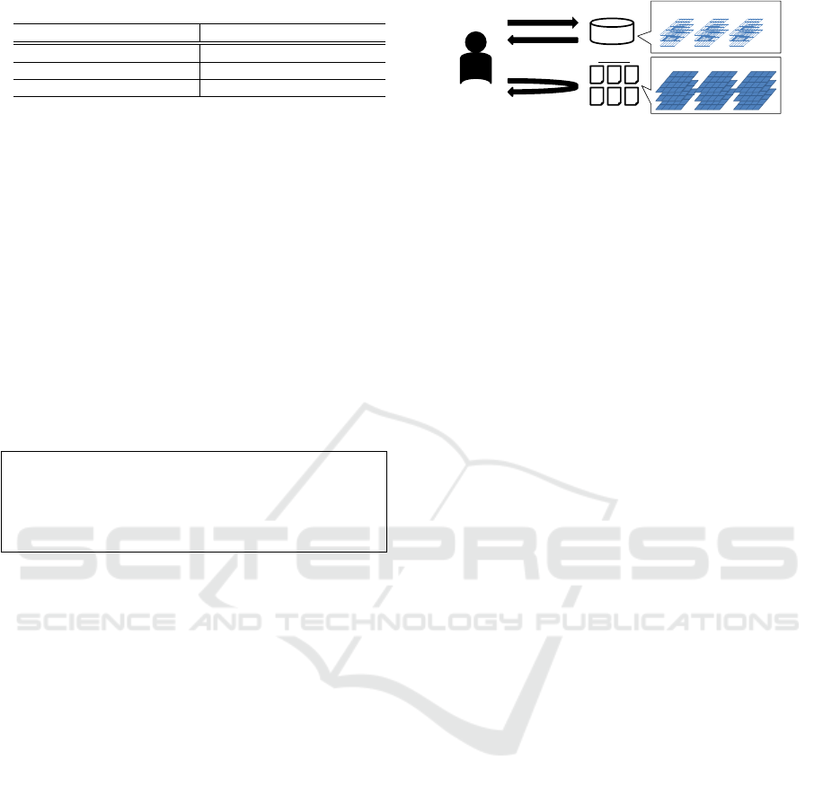
Table 1: Schema of a distribution data.
Name Description Name Description
id ID of records y y coordinate value
did ID of distributions t time (hour)
x x coordinate value v the quantity
De Roo, 2000), and so on(Park et al., 2005)(Hof-
stra et al., 2009)(the European Climate Assessment
& Dataset project team, 2016). Many algorithms
to generate grid data from a point dataset have also
been proposed (Silverman, 1986) (Seaman and Pow-
ell, 1996)(Asahara et al., 2015). This implies that
such grid data are useful for various use cases.
Table 1 lists items of a table-managing grid data
modeling a quantity distribution. Every distribution,
having an identifier of a distribution (denoted as did),
consists of multiple records. The records have loca-
tion data (denoted as x,y), time data (denoted as t)
and the quantity value denoted as v.
Using spatio-temporal-indexing technologies, we
can quickly retrieve the quantity data any place any
time. A query, for example, is following.
select di d from di s t rib u t ion w h e r e
(x b etween 10 an d 20)
an d ( y b e t w e e n 10 and 2 0)
an d ( t b e t w e e n 10 and 1 5)
an d ( v > 100.0)
The result of this query is a list of dids, the v of which
in a square 10 < x < 20 and 10 < y < 20 was more
than 100.0 in between 10:00 and 15:00. A usecase of
the query is a hypothesis test of “the sales figures of
a store in 10 < x < 20 and 10 < y < 20 was quite
high during heavy rain (more than 100mm).” The
query is very simple. The overhead of managing re-
lational database systems (RDBMS), however, is ex-
tremely large due to the huge number of records in the
database (e.g. 14 billion records as discussed above).
2.2 Related Works
Many indexing technologies for spatio-temporal
point data have been proposed (Koubarakis
et al., 2003)(Hayashi et al., 2015)(Haynes et al.,
2015)(Theodoridis et al., 1998). These technologies
are applicable to the quantity distribution datasets
because the data can be handled as point data.
However, the number of records makes problems of
the storage cost as discussed above. Thus methods
to reduce DB records without loss of accuracy are
required from the aspect of costs.
Additionally many indexing techniques for raster
data are proposed(Zhang et al., 2010)(Pajarola and
Widmayer, 1996) and implemented(Shyu et al.,
2007). The scientific array databases(Oracle,
DB
Spatio-temporal
conditions
Filenames
Data files
Sparse datasets
Files
Original datasets
User
Figure 1: Sparse-data-based system.
2014) moreover are produced to handle such grid
datasets. SciDB(Stonebraker et al., 2013) and Ras-
daman(Baumann et al., 1999) are well-known soft-
ware to manage array data. For such systems, SQL
Multidimensional Array(International Standard Orga-
nization, ) for queries to array data was standarized.
Most of them are based on the raster boundaries and
its hierarchical structure, such as R-trees and quad
trees but data themselves are not reduced. Note that
these methods and a record reduction might be used
together to create a synergy effect. For example,
the reduced records can be retlieved with a spatio-
temporal indexing technology.
2.3 Approach
As a solution to the problem, our method reduces the
number of records without loss of information. Figure
1 illustrates an overview of a sparse-data-based sys-
tem. A user of this system requests the database (la-
beled as DB in the figure) for distributions satisfying
a condition. The user obtains filenames correspond-
ing to the did as “candidates”. The user can thus find
distribution data files (e.g. NetCDF (Open Geospa-
tial Consortium, 2010) files). The user finally obtains
the desired distribution data files. Note the DB is not
used for finding the final results. The DB manages a
rough distribution for finding candidates. Therefore,
the number of records in the database can be smaller
than that of the original records. The user will require
various queries without programming. SQL, which
is one of the most frequently used languages, is use-
ful for such users. Thus, the process to request the
database should be completely written in SQL, that is,
the database should be implemented with a RDBMS.
Another point is precision. Generally, most mea-
surements include errors due to observation. This fact
suggests that the users of the system can accept small
errors. Although some users might require the most
accurate information, the original dataset should be
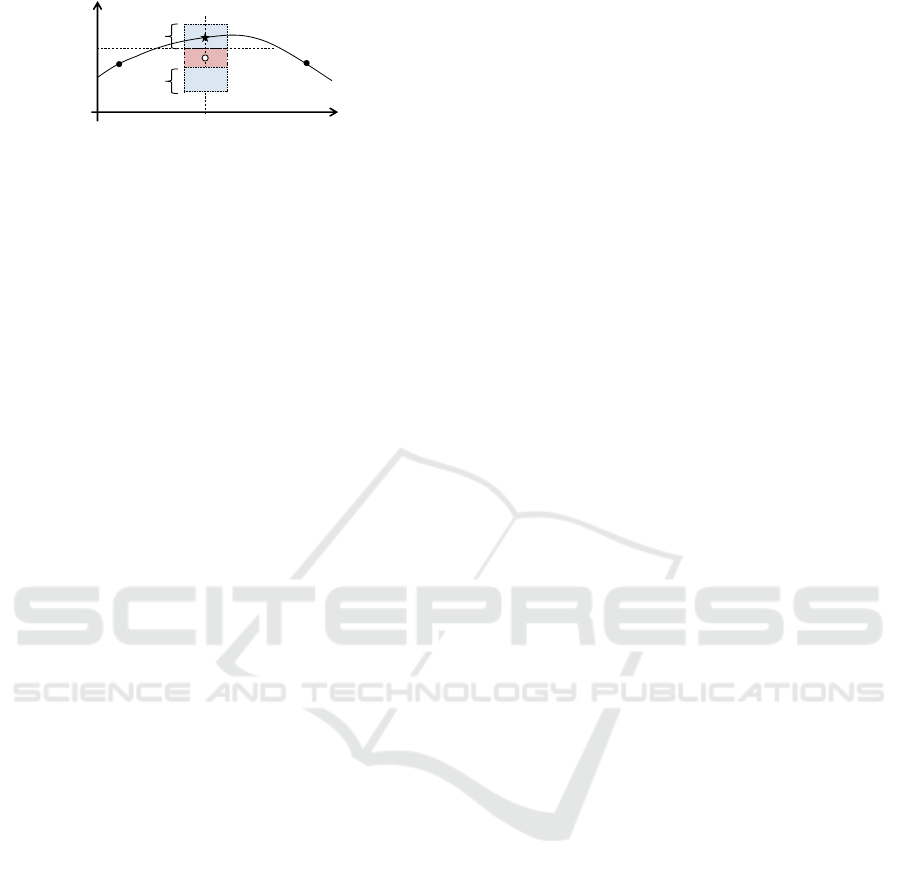
accessible. Figure 2 illustrates the mechanism to re-
trieve the original data. The vertical axis is v and
the horizontal axis is x, in the illustration. The solid
curve represents distribution of the original dataset.
The white circle shown in the center of the graph rep-
resents the roughly estimated v at x
i
and the square
GISTAM 2017 - 3rd International Conference on Geographical Information Systems Theory, Applications and Management
210
v(x)
x
x
i
v
i
ε
ε
Figure 2: Query with error ε.
colored by red shows the range of a query (data in the
red region should be retrived). Because the estimated
value is not accurate, the actual value represented by
the black star is out of the red region. However, ba-
cause the error is less than ε, distance between the
white circle and the black star is less than ε. Thus the
actual value can be obtained if the query region was
set as the red region plus the blue region which rep-
resents the range of which is added by ε. As shown
in this example, even if the data have an error ±ε,
the query condition with ±ε hits all possible distribu-
tions. The result might include unnecessary distribu-
tions, though they can be removed after fetching the
original datasets. Therefore, the database can accept
a small error less than a preset threshold denoted as ε.
2.4 Contribution
In summary of the last section, the distribution data in
the database should be fewer than the original dataset.
Additionally, a query to obtain one of the distribution
data should be written in SQL for usability. Alterna-
tively the distribution data may be imprecise. Thus,
a small dataset having information to reconstruct the
original dataset should be managed in a RDBMS.
One of the naive approaches to reduce the num-
ber of data is random sampling, which involves ran-
domly removing some of the data, so precision can-
not be controlled. Another naive approach involves
using the averages of multiple data. However, pre-
cisions of sparse representations using such methods
are quite low. Generally the reconstruction with fewer
information will be difficult, therefore the records in
RDBMS cannot be recuded so much to keep informa-
tion enough to the reconstrucion.
We therefore propose a method using a sparse
representation generated with kernel regressions(John
Shawe-Taylor, 2004). A kernel regression, which is
defined as a regression using a kernel trick, is com-
monly used for prediction, interpolation, and so on.
Inputs of a kernel regression are point-value pairs. A
kernel regression constructs a non-linear function to
predict values at such points.The basic concept of the
kernel trick is that an imaginary non-linear transfor-
mation is assumed to find a linear regression func-
tion. The formula of a linear regression function can
be changed to another formula using only similari-
ties between input data. Therefore, all that needs to
be defined is the similarity formula, which is called a
kernel function. The regression function is very pre-
cise; thus, the original dataset can be accurately re-
constructed. Therefore, a highly sparse representation
of a quantity distribution can be derived using a kernel
regression.
3 SPARSE REPRESENTATION
GENERATED WITH KERNEL
REGRESSION
3.1 Kernel Ridge Regression
Many kernel regressions have been proposed such as a
support vector regression (SVR) (Vapnik et al., 1997).
The proposed method uses a kernel ridge regression,
which is equivalent to Kriging (Kbiob, 1951)(Press
et al., 2007) used for geostatistics. A ridge regression
is a linear regression method based on “least square
mean errors”. The formula of the ridge regression is
non-linearized with the kernel trick to obtain the ker-
nel ridge regression. The regression result denoted as
v(x) is written as follows.
v(x) =
v
1
v
2
···
(G + σI)
−1
κ(x
1
, x)
κ(x
2
, x)
.
.
.
(1)
where I is a unit matrix, σ is a parameter, and G is
called ‘Gram matrix.’ G is defined as
G =
κ(x
1
, x
1
) κ(x
1
, x
2
) · ··
κ(x
2
, x
1
) κ(x
2
, x
2
) · ··
.
.
.
.
.
.
.
.
.
. (2)
The κ(·, ·) is a kernel function to evaluate the simi-
larity of two data. Note that v(x
i
) always equals v
i
(i.e. the product of G
−1
and (κ(x
1
, x
2
), κ(x
2
, x
2
), ··· )
is (0, 1, 0, ·· ·) ) when σ = 0. Thus, v(x) with σ = 0
can completely reconstruct the original distribution if
all of the original data are involved by v(x). This en-
sures the lower bound of the error as 0. Therefore,
any threshold ε can be acceptable.
3.2 Sparse Representation Generation
The algorithm of our proposed method to generate a
sparse representation dataset is shown in Algorithm 1.
The initial dataset is set to a dataset including only the
point at the origin (0,0) for simplifying the algorithm.
It can be set to another small dataset though the choice
Quantity Distribution Search using Sparse Representation Generated with Kernel-based Regression
211

Algorithm 1: Naive sparse representaion generation.
Data: Original dataset {x
i
}, preset threshold ε and
parameter θ
Result: sparse representation {x
0
i
} and weights {w
i
}
1 begin
2 initialize sparse dataset {x
0
i
} from {x
i
}
3 initialize G
−1
with formula (2) using {x
0
i
}
4 while the number of {x
0
i
} 6= the number of {x
i
}
do
5 find the maximal-error point out from {x
i
}
with formula (1) using G
−1
6 (point x
m
, error e) ← the maximal-error
point
7 if e ≤ ε then
8 end this loop
9 Append x
m
to {x
0
i
}
10 update G
−1
with formula (2) using {x
0
i
}
11 return {x
0
i
} and {w
i
}
does not make significant effect because much more
data will be added. An iteration is carried out at the
next step. If maximal error of the generated func-
tion is lower than the preset threshold ε, the iteration
should be finished to output the dataset as the sparse
representation. If the maximal error is even more
than ε, another data needs to be added to improve ac-
curacy. The data with the maximal error (hereafter,
called the max-error point) is selected as the data to
be added because it lowers the maximal error. The
maximal error in the next iteration is thus automati-
cally changed, so another data will be selected to be
added in the next iteration. The kernel ridge regres-
sion result completely reproduces the input data as
mentioned above. The maximal error will be 0 after
adding all the original data to the sparse representa-
tion. Therefore, the sparse representation is equiva-
lent to the original dataset in the worst case.
An inverse matrix of Gram matrix G
−1
is calcu-
lated in the iteration. The calculation takes much time
because the computational complexity is o(n
3
) (n is
the dimension of G, that is, the number of data). The
recurrence formula is thus used for accelerating the
calculation. The formula of a Gram matrix using n
data, G
n
, is written as
G
n+1
=
G
n
c
n+1
c
T
n+1
κ(x
n+1
, x
n+1
)
, c
n
=
κ(x
1
, x
n
)
.
.
.
!
.
(3)
By using the formula for the inverse of a block matrix
A B
C D
−1
=
A
−1
+ A
−1
BECA
−1
−A
−1
BE
−ECA
−1
E
(4)
E = (D −CA
−1
B)
−1
(5)
the following formula is obtained.
G
−1
n+1
=
1
s
sG
−1
n
+VV
t
−V
−V
t
1
, (6)
where
s = κ(x
n+1
, x
n+1
) − c
T
n+1
G
−1
n
c
n+1
(7)
V = G
−1
n
c
n+1
. (8)
The algorithm is quite similar to the Douglas-
Peucker algorithm (David and Thomas, 1973) known
as a simplification algorithm for a polyline. The
Douglas-Peucker algorithm has an issue regarding the
computation time in finding the furthest point (Hersh-
berger and Snoeyink, 1994). Similarly, the algorithm
of the proposed method to generate a sparse represen-
tation also has an issue regarding processing speed in
finding the maximal-error point. An error of a point,
which is defined as |v(x
i
)−x
i
|, includes the evaluation
of v(x). Calculation time for this evaluation will be
huge due to the number of original data because it is
convolution of sparse representation for all data of the
original dataset. Accordingly the convolution should
be carried out on a small region to reduce calculation
time. In addition, doubly evaluated v(x) should be
sorted out, that is, v(x) values calculated in the for-
mer iteration are suitable for the later iteration until
the values are changed.
3.3 Kernel Functions
Various kernel functions are already known such
as Gaussian kernel and polynomial kernel function,
which affect an infinite region. The algorithm of the
proposed method, however, has a problem caused by
the huge number of the original data if the kernel
function widely affects v(x). So the polynomial ker-
nel function is suitable for the proposed method, de-
scribed as
κ(x
i
, x
j
) =
1 −
|x
i
−x
j
|
2
θ
d
(
|x
i
−x
j
|
θ
< 1)
0 (
|x
i
−x
j
|
θ
> 1)
, (9)
where θ is a parameter to be set manually. The func-
tion is an exponent of a quadratic function normally
used in density estimation. The function, called expo-
nential circular kernel (ECK) hereafter, is applicable
to the kernel ridge regression.
The effect of the ECK is limited in a circle the
radius of which is θ. Hence, the calculation of v(x) is
shortened.
v(x) =
∑
|x
i
−x|<θ
w
i
κ(x
i
, x) (10)
GISTAM 2017 - 3rd International Conference on Geographical Information Systems Theory, Applications and Management
212

Algorithm 2: Sparse representaion generation.
Data: Original dataset {x
i
}, preset threshold ε and
parameter θ
Result: sparse representation {x
0
i
} and weights {w
i
}
1 begin
2 initialize sparse dataset {x
0
i
} from {x
i
}
3 initialize G
−1
with formula (2) using {x
0
i
}
4 initialize {w
i
} with formula (11) using G
−1
and
{x
0
i
}
5 initialize heap H for {x
i
} with formula (10)
using ({x
0
i
},{w
i
})
6 while the number of {x
0
i
} 6= the number of {x
i
}
do
7 (point x
m
, error e) ← pull the maximal-error
point out from H
8 if e ≤ ε then
9 end this loop
10 Append x
m
to {x
0
i
}
11 incrementally update of G
−1
and {w
i
} with
formula (6)
12 for each x with |x −x
m
| < θ do
13 update error |x −v(x)| of x in H with
formula (10) using ({x
0
i
}, {w
i
})
14 maintain heap structure of H for x
15 return {x
0
i
} and {w
i
}
where w
i
is defined as
w
i
=
∑
|x
i
−x
j
|<θ
v
j
G
−1
i, j
. (11)
Parameter θ shown in the ECK accordingly indicates
the distance in which the quantity of the distribution
does not change much, that is, the range of blur. d
indicates the sharpness of the distribution. The pa-
rameters should be tuned for the distribution with pa-
rameter tuning methods such as cross validations.
Furthermore, the step to find the maximal-error
point can be accelerated with ECK, as shown in Al-
gorithm 2. The code shows a function to generate a
sparse representation of the given dataset denoted by
the original dataset {x
i
}. A minimal dataset {x
0
i
} is
initially set to be very small and the inverse matrix
of the Gram matrix is calculated only once at the ini-
tialization. The {x
0
i
} is enlarged during the iteration
and G
−1
is incrementally updated with formula (6).
When a new data is added, v(x) only at the θ-radius
region around the data is changed. Therefore, for the
other v(x)s, the calculation results at the former iter-
ations are re-usable. A well-known heap-sort algo-
rithm is suitable for finding the maximal-error point.
Namely, all pairs of errors |y
i
− v(x
i
)| and data x are
initially calculated and managed in a max heap H.
The maintenance of H (e.g. the loop at line num-
ber 12 in Algorithm 2) is limited around the maximal-
error point due to the ECK. The maximal-error point
can be easily removed from the heap because the top
of the heap is the maximal-error point. After adding
the maximal-error point to the sparse representation,
the |y
i
− v(x
i
)| to be updated are calculated and re-
flected to the data in the heap. The heap structure can
be maintained in O (n logn) runtime, so the process to
find the maximal-error point is quite fast.
Thus, the sparse representations did, x, y, t, and w
have to be stored in a relational database. The recon-
struction can be implemented with SQL as follows.
select sid , sum (w * pow (1.0
- d i st ([{ x0 , y0 }] ,{ x , y } ) /[ theta ]) ,[ d ])
fro m dist r i but i o n
where di s t ([{ x0 , y0 }] ,{x , y }) < [ theta ]
group by sid
where dist(·,·) is a function to calculate the Euclid-
ian distance between two points and [ ] indicates the
query condition given by the user.
4 EXPERIMENTS
To evaluate how small a sparse representation dataset
generated with the algorithm of the proposed method
is, we conducted an experiment using actual quantity-
distribution data.
The dataset, summarized in Table 2, contains the
DEM data of Shizuoka prefecture of Japan (the ID
of this region is 5238)(Ministry of Land, Infrastruc-
ture, Transport and Turism, 2014). The region was
split into 320 × 320 grids to represent the distribu-
tion of the ground surface height, where the grid size
was around 250 m. The dataset consisted of 102,400
records, including the invalid data on the height of
the ocean. After removing the ocean data, there were
74,663 records - this was the baseline. The computer
used for the experiment had an Intel Corei-7 3770K
3.5-GHz CPU and 16-GB RAM. The sparse repre-
sentation generation algorithm was implemented with
Java, and JDK 1.8.0 update 31 on OS Windows 7 was
used as the environment to run it.
To exhibit how the parameter ε works, two param-
eter settings were tested in the experiment. As the
first setting, ε was set to 125 m; θ was set to 5 (1250
m); degree of the ECK was d = 2. The calculation to
generate the sparse representation took 383.8 s. The
threshold was set to 250 m; θ was set to 5 (1250 m);
and degree of the ECK d = 2. The calculation time
was 74.9 seconds. The results indicate that the thresh-
old setting is crucial for performance.
The datasets were imported into PostgreSQL 9.2
database and a multicolumn b-tree index to x and y
Quantity Distribution Search using Sparse Representation Generated with Kernel-based Regression
213
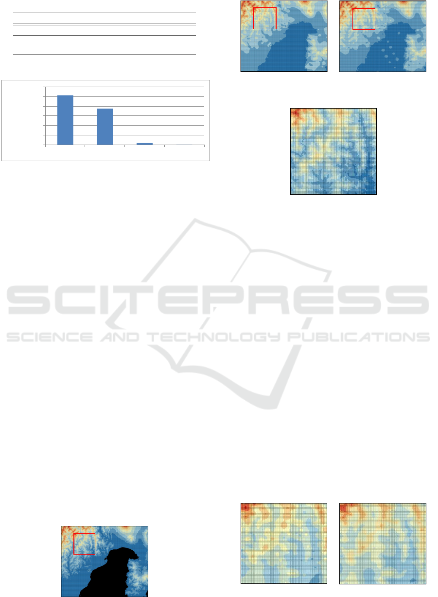
Table 2: Overview of the DEM dataset.
Name description
Size 3.8MB on RDBMS
# of records 102,400 records
74,663 records for ground surface
Region ID 5238 around Shizuoka Pref.
102400
74663
3413
888
0
20000
40000
60000
80000
100000
120000
All data
Land only
ε=125
ε=250
# of Data
Figure 3: The number of records.
is generated to evaluate the performance to manage
the original data. Figure 3 plots the number of the
sparse representations and that of the original data.
The table data size of the original dataset consist-
ing of 74,663 records was 3.8MB and the index size
was 3.0MB. The sparse representation with ε =125m
consists of 2,898 records (3.9% of Land only data).
The table data size was 152KB; index datasize was
168KB. The sparse representation ε =250m consists
of 1,133 records (1.5%); the table data size of Post-
greSQL was 64KB; index datasize was 64KB.
The original dataset reconstruction was also car-
ried out for the same dataset to confirm the quality.
For the sparse dataset of ε = 125 and ε = 250, a re-
construction query of one grid was finished in 12 ms.
The query for the record to the original dataset fin-
ished in 11 ms. This shows data reconstruction im-
plemented by SQL is not slow in obtaining a recon-
structed dataset. Figures 4, 5(a), and (b) respectively
present the original distribution, images reconstructed
with sparse representation with ε = 125 m, and that
with sparse representation with ε = 250 m. They are
quite similar but the details are not. Figures 6 and 7
compare close-up images of the regions marked with
red squares in Figures. 4 and 5, respectively. The
original dataset had small irregularities, which were
smoothed in the sparse representations. The sparse
representation with 250 m was rougher than that with
125 m. In addition to the conditions, ε = 375 and
ε = 500 were also tested; the number of records was
Figure 4: Original dataset.
(a) 125m (b) 250m
Figure 5: Sparse representations.
Figure 6: Close-up image of the original dataset.
293 and 148; the processing time were 20.4 s and 10.3
s, respectively. The results shows that the accuracy
and the speed of the algorithm of the proposed method
sensitively depend on ε. Therefore, ε should be used
to precisely reconstruct the original dataset.
Figures 8 illustrate the sparse representation and
close-up image. The red triangles are the location of
the sparse dataset. Fewer data were on a flat region
and more data were on irregular regions. Many data
were put along the coastline because elevations of the
coastline indicate extreme gaps in land and sea lev-
els. This tendency suggests that the proposed method
works well to remove unnecessary flat data.
Additionally the parameters used in the proposed
method are changed to clarify the effects. Figure 9
plots the number of records by various θ (ε was set
to 250). When θ is 10, the number of records was
largest. Because θ gives the range of the effect by the
ECK, more records were needed for covering all re-
gions when θ was small. Figure 9 plots the precisions
for each θ. The vertical axis of the graph represents
the averaged errors with the sparse representations.
More sparse representation was expected to give ac-
curate results though the larger θ gave precise results.
(a) 125m (b) 250m
Figure 7: Close-up images of sparse representations.
GISTAM 2017 - 3rd International Conference on Geographical Information Systems Theory, Applications and Management
214
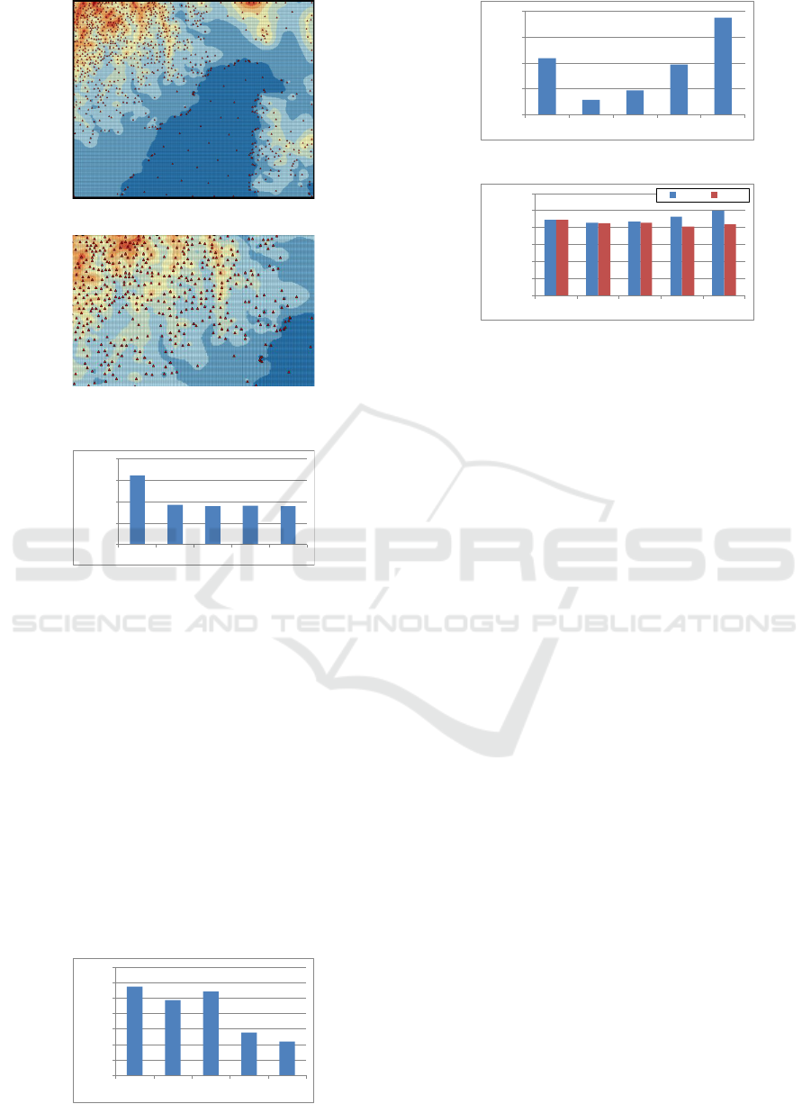
(a) overview
(b) close-up image
Figure 8: Data of sparse representation.
1604
924
889
903
888
0
500
1000
1500
2000
θ=10
θ=20
θ=30
θ=40
θ=50
# of Data
Figure 9: The number of records by θs.
The proposed algorithm is based on the max error, so
sparseness of the sparse representation is not corre-
lated to the accuracy. Figure 11 plots the processing
times for each θs. The fastest setting was θ = 20.
Generally if θ is smaller, more records are required as
disscussed above. Thus, when a small θ is used, the
processing time is longer. However, θ is the range of
the effect by the ECK also. That is, the region to be
calculated might be small when a small θ is used. The
fact implies that the processing time is shorter. These
two factors are balanced at θ=20 in the case.
Moreover graphs shown in Figure 12 plot the
number of records for each d of ECK. When θ = 30,
d = 3 gave the minimal number of records; d = 5 gave
the minimal number of records when θ = 50. Gener-
ally large d gives a sharp ECK. So d should be tuned
62
64
66
68
70
72
74
76
θ=10
θ=20
θ=30
θ=40
θ=50
Errors [m]
Figure 10: The precisions by θs.
0
20
40
60
80
θ=10
θ=20
θ=30
θ=40
θ=50
Processing Time [s]
Figure 11: Processing Time for each θ.
0
200
400
600
800
1000
1200
d=2
d=3
d=4
d=5
d=6
# of Data
θ=30
θ=50
Figure 12: The number of records by θs.
to get the minimal number of records. However the
best d depends on θ. The fact implies that both d
and θ should be selected carefully to get the smallest
sparse representation.
5 CONCLUSIONS
We proposed a method for managing quantity distri-
butions. With this method, a sparse representation of
a quantity distribution is derived using kernel ridge
regression. The sparse representation dataset is small
enough to handle by using RDBMSs without high
cost. An advantage of the proposed method is that
the reconstruction can be written in SQL. Therefore
the proposed method can easily provide drill-down
functions. We experimentally applied the algorithm
of the proposed method to DEM data. As a result, the
number of records was reduced to less than 1/10 (e.g.
3.9%) that of the original number. In addition, the
data retrieval performance was comparable with that
for the original dataset. This shows that the proposed
method can reduce records without loss of speed.
SVR, of which formula is more sparse than that of
kernel ridge regression, is also well known. A SVR-
based sparse representation thus might be more com-
pact. A reason why the algorithm of the proposed
method uses kernel ridge regression is that the kernel
ridge regression ensures accuracy if σ = 0. Support
vector regression does not output such accurate rep-
resentation; thus, an algorithm to generate an SVR-
based sparse representation is for future work.
Quantity Distribution Search using Sparse Representation Generated with Kernel-based Regression
215

REFERENCES
Asahara, A., Hayashi, H., and Kai, T. (2015). Moving
point density estimation algorithm based on a gener-
ated bayesian prior. ISPRS International Journal of
Geo-Information, 4(2):515–534.
Bates, P. D. and De Roo, A. (2000). A simple raster-based
model for flood inundation simulation. Journal of hy-
drology, 236(1):54–77.
Baumann, P., Dehmel, A., Furtado, P., Ritsch, R., and Wid-
mann, N. (1999). Spatio-temporal retrieval with ras-
daman. In VLDB, pages 746–749.
Christensen, J. H., Kjellstr
¨
om, E., Giorgi, F., Lenderink, G.,
Rummukainen, M., et al. (2010). Weight assignment
in regional climate models. Climate research (Open
Access for articles 4 years old and older), 44(2):179.
David, H. D. and Thomas, K. P. (1973). Algorithms for the
reduction of the number of points required to represent
a hne or its caricature. The Canadian Cartographer,
10(2):112–122.
Hayashi, H., Asahara, A., Sugaya, N., Ogawa, Y., and
Tomita, H. (2015). Spatio-temporal similarity search
method for disaster estimation. In 2015 IEEE Inter-
national Conference on Big Data (Big Data), pages
2462–2469. IEEE.
Haynes, D., Ray, S., Manson, S. M., and Soni, A. (2015).
High performance analysis of big spatial data. In
2015 IEEE International Conference on Big Data (Big
Data), pages 1953–1957. IEEE.
Hershberger, J. and Snoeyink, J. (1994). An o(nlogn) imple-
mentation of the douglas-peucker algorithm for line
simplification. In Proceedings of the Tenth Annual
Symposium on Computational Geometry, SCG ’94,
pages 383–384, New York, NY, USA. ACM.
Hofstra, N., Haylock, M., New, M., and Jones, P. D.
(2009). Testing e-obs european high-resolution grid-
ded data set of daily precipitation and surface tem-
perature. Journal of Geophysical Research: Atmo-
spheres, 114(D21).
International Standard Organization. ISO IEC CD
9075-15 Information technology – Database
languages – SQL – Part 15: Multi dimen-
sional arrays. http://www.iso.org/iso/home/store/
catalogue tc/catalogue detail.htm?csnumber=67382.
John Shawe-Taylor, N. C. (2004). Kernel Methods for Pat-
tern Analysis. Cambridge University Press.
Kbiob, D. (1951). A statistical approach to some basic mine
valuation problems on the witwatersrand. Journal of
Chemical, Metallurgical, and Mining Society of South
Africa.
Koubarakis, M., Sellis, T., Frank, A. U., Grum-
bach, S., G
¨
uting, R. H., Jensen, C. S., Lorent-
zos, N., Manolopoulos, Y., Nardelli, E., Pernici,
B., et al. (2003). Spatio-temporal databases:
The CHOROCHRONOS approach, volume 2520.
Springer.
Ministry of Land, Infrastructure, Transport and Turism
(2014). National Land Numerical Information Data.
http://nlftp.mlit.go.jp/ksj-e/index.html.
Open Geospatial Consortium (2010). OGC Net-
work Common Data Form (NetCDF) Core En-
coding Standard version 1.0 (10-090r3). http://
www.opengeospatial.org/standards/netcdf.
Oracle (2014). Oracle Spatial and Graph GeoRaster,
ORACLE WHITE PAPER SEPTEMBER 2014.
http://download.oracle.com/otndocs/products/spatial/
pdf/12c/oraspatialfeatures 12c wp georaster wp.pdf.
Pajarola, R. and Widmayer, P. (1996). Spatial index-
ing into compressed raster images: how to answer
range queries without decompression. In Multimedia
Database Management Systems, 1996., Proceedings
of International Workshop on, pages 94–100. IEEE.
Park, S., Bringi, V., Chandrasekar, V., Maki, M., and
Iwanami, K. (2005). Correction of radar reflectiv-
ity and differential reflectivity for rain attenuation
at x band. part i: Theoretical and empirical ba-
sis. Journal of Atmospheric and Oceanic Technology,
22(11):1621–1632.
Press, W. H., Teukolsky, S. A., Vetterling, W. T., and Flan-
nery, B. P. (2007). Numerical Recipes 3rd Edition:
The Art of Scientific Computing. Cambridge Univer-
sity Press, New York, NY, USA, 3 edition.
Seaman, D. E. and Powell, R. A. (1996). An evaluation
of the accuracy of kernel density estimators for home
range analysis. Ecology, 77(7):2075–2085.
Shyu, C.-R., Klaric, M., Scott, G. J., Barb, A. S., Davis,
C. H., and Palaniappan, K. (2007). Geoiris: Geospa-
tial information retrieval and indexing systemContent
mining, semantics modeling, and complex queries.
IEEE Transactions on geoscience and remote sensing,
45(4):839–852.
Silverman, B. W. (1986). Density Estimation for Statistics
and Data Analysis. Chapman and Hall/CRC.
Stonebraker, M., Duggan, J., Battle, L., and Papaem-
manouil, O. (2013). Scidb DBMS research at M.I.T.
IEEE Data Eng. Bull., 36(4):21–30.
the European Climate Assessment & Dataset project team
(2016). European Climate Assessment & Dataset,
Daily Data. http://www.ecad.eu/dailydata/index.php.
Theodoridis, Y., Sellis, T., Papadopoulos, A. N., and
Manolopoulos, Y. (1998). Specifications for effi-
cient indexing in spatiotemporal databases. In Scien-
tific and Statistical Database Management, 1998. Pro-
ceedings. Tenth International Conference on, pages
123–132. IEEE.
Vapnik, V., Golowich, S. E., Smola, A., et al. (1997). Sup-
port vector method for function approximation, re-
gression estimation, and signal processing. Advances
in neural information processing systems, pages 281–
287.
Zhang, J., You, S., and Gruenwald, L. (2010). Indexing
large-scale raster geospatial data using massively par-
allel gpgpu computing. In Proceedings of the 18th
SIGSPATIAL International Conference on Advances
in Geographic Information Systems, pages 450–453,
New York, NY, USA. ACM.
GISTAM 2017 - 3rd International Conference on Geographical Information Systems Theory, Applications and Management
216
