Solid Waste Collection Routing Optimization using Hybridized

Modified Discrete Firefly Algorithm and Simulated Annealing

A Case Study in Davao City, Philippines

Cinmayii Manliguez

1,2

, Princess Cuabo

, Ritchie Mae Gamot

and Kim Dianne Ligue

Department of Mathematics, Physics, and Computer Science, University of Philipines, Philipines

Phil-LiDAR 1.B.13 LiDAR Data Processing and Validation in Mindanao: Davao Region

College of Science and Mathematics, University of the Philippines Mindanao,

Davao City, 8022, Philippines,

Keywords: Garbage Collection, Routing Optimization, Travelling Salesman Problem, Discretization, Metaheuristics.

Abstract: Modified Discrete Firefly - Simulated Annealing (MDF-SA) Algorithm was used to solve travelling salesman

problem (TSP) using the tanh function for discretization. MDF-SA was tested on four (4) data instances from

TSPLIB and the Davao City solid waste collection routing system. The objective of this study is to evaluate

and compare MDF-SA with MDFA in terms of running time and solution quality. The data set selected from

the TSPLIB are ST70, PR152, GR431, and TS225. The Davao City solid waste collection routing system is

used in the hopes of finding a better solution from the current. Results show that MDF-SA and MDFA perform

almost equally well on the data sets PR152 and GR43. MDFA performs better on using the TS225 data set,

but MDF-SA performs much better on ST70. In general, the hybrid algorithm has produced better route

system quality of the Davao City solid waste collection than the MDFA.

1 INTRODUCTION

Solid waste management is becoming critical in the

current setting due to the escalating urbanization and

population growth in a location, coupled with

increasing environmental concerns (Awad et al.,

2001). Davao City, for instance, is the most densely

inhabited and highly industrialized city in Region XI

having an approximately 1.63 million residents in

2015 (Philippine Statistics Authority, 2015). As a

result, the volume of waste collected per day

increased by 100% since 2013 driving the city

government to spend about ₱13 million for the

monthly rental of a hundred garbage trucks (Carillo,

2016). This situation poses a good basis for the

importance of optimization in the process of garbage

collection like routing.

The routing problem is one of the main

components of garbage collection. The goal of

optimizing the route for solid waste collection is to

minimize the cost at a desired level of service.

According to Karadimas et al. (2007), at most 80% of

solid waste disposal budget is spent on collection.

Therefore, a small improvement in the collection

operation can result to a significant saving in the

overall cost.

This study explores the possibility of hybridizing

the Modified Discrete Firefly Algorithm (MDFA)

and Simulated Annealing (SA) Algorithm in solving

the solid waste collection routing. Specifically, this

study aims to:

1. Evaluate the performance of Modified

Discrete Firefly with Simulated Annealing

(MDF-SA) algorithm in terms of running

time and solution quality (distance);

2. Evaluate and compare the performance of

MDF-SA algorithm with that of MDFA in

terms of running time and solution quality

using four benchmark data instances (PR152,

ST70, TS225, and GR431)

3. Evaluate the performance of MDFSA

algorithm as applied to solid waste

collection in terms of running time and

solution quality (distance units), and the

2014 Davao City solid waste collection

routing system); and

4. Compare MDF-SA’s performance (solution

quality) with the existing total distance taken

to complete the solid waste collection

Manliguez C., Cuabo P., Gamot R. and Ligue K.

Solid Waste Collection Routing Optimization using Hybridized Modiﬁed Discrete Fireﬂy Algorithm and Simulated Annealing - A Case Study in Davao City, Philippines.

DOI: 10.5220/0006322500500061

In Proceedings of the 3rd International Conference on Geographical Information Systems Theory, Applications and Management (GISTAM 2017), pages 50-61

ISBN: 978-989-758-252-3

routing system in the city of Davao,

Philippines.

This study is limited to the evaluation of the

introduction of standard Simulated Annealing

algorithm to Modified Discrete Firefly algorithm, as

well as the evaluation of the hybrid’s performance

when it is applied to known TSP benchmark data sets

specifically the PR152, ST70, TS225, GR431, and the

garbage collection routing system in the city of Davao,

Philippines.

In this paper, a background of solid waste

collection, the area of study and the algorithms are

discussed first. Next is the methodology of the study,

followed by the results and discussion, and lastly, the

summary and conclusions.

2 RELATED LITERATURE

Davao City, one of the largest city in the world, has a

land area of approximately 244,000 hectares and is

located in Regions 11 or Southern Mindanao. The city

is lying in the grid squares with latitude of 6 degrees

58 minutes to 7 degrees 34 minutes North, and

longitude of 125 degrees 14 minutes to 125 degrees

40 minutes East. The city is bounded by Davao

Province on the north, Davao Province and Davao

Gulf partly on the east, Davao del Sur on the south,

and North Cotabato on the west (City of Davao,

2011a). Coming from Manila, Davao City Proper

goes southeast and is approximately 946 aerial

kilometers.

The strategic location of Davao City made it the

regional trade center in Southern Mindanao, was

developed as international trade center to the

Southern Pacific, and Southern Gateway of the

neighboring countries like Brunei, Indonesia,

Malaysia, Australia, and others (City of Davao,

2011b). There are three congressional districts in the

city, and 11 administrative districts. Davao City

Environmental and Natural Resources Office

summarizes the demography on environmental

services from 2006 to 2010 in Table 1.

2.1 Nondeterministic Polynomial-Time

(NP) Complete Problems

Nondeterministic Polynomial-time complete

problems from theoretical computer science is a very

intriguing (Dasgupta et al., 2006) and tantalizing class

of problems because of their reduction property,

making every problem equally difﬁcult or easy to

solve (Jensen, 2010). To be able to obtain feasible

solutions that are short and easy-to-recognize,

suitable constraints have to be introduced (Kann,

2000). According to Grom (2010), a problem x that is

in NP is also in NP-Complete if and only if every

other problem in NP can be quickly (i.e. in

polynomial time) transformed into x. A few examples

of NP-complete problems include Multiprocessor

Scheduling Comparative Divisibility, Satisfiability

with 3 literals per clause (3-SAT), and traveling

salesman problem (Ruiz-Vanoye et al., 2011).

2.1.1 Travelling Salesman Problem

The travelling salesman problem (TSP) is one of the

most studied discrete optimization problems

(Bookstaber, 1997). Although TSP is difficult to

Table 1: Demography on Environmental Services 2006-2010 of Davao City (City of Davao, 2011b).

Indicato

2006 2007 2008 2009 2010

Average Volume of garbage

disposed daily, cu. M.

946.51 997.14 996.03 1167 1189

Number of hauling trucks

utilized

43 75 80 83 80

Number of Garbage

Collectors

280 714 714 714 360

Frequency of Collection Daily Daily Daily Daily Daily

Dumping Site (location) Brgy. New Carmen,

Tugbok District

Barangay Lacson,

Calinan District

Barangay Lacson,

Calinan District

Barangay Lacson,

Calinan District

Brgy. Lacson, Calinan

Dist. and Brgy.

Carmen Tugbok Dist.

Other garbage disposal

practices

Burning,

dump in pit,

composting

Burying Composting Composting Composting

Garbage Sources, %

Residential, Commercial,

Industrial

- 83 83 83 83

Market - 15 15 15 15

Canals/garden waste/cut

trees

- 2 2 2 2

solve especially with large number of cities, it is still

very popular because aside from it is easy to

formulate, it has a large number of applications.

Lin (1965) defined TSP as a problem of a

salesman who needs to visit each city only once of the

N given cities. The salesman can start from any city

but should return to that same city. One critical

consideration in the solution is that the route or tour

that the salesman must take must have the minimum

distance. Distance traveled may be replaced with

other notions such as time, cost, etc. The salesman

must know the distances of travelling between each

pair of cities (Poort, 1997).

TSP may be represented as a weighted graph. The

nodes of the graph represent the cities and the edges

represent the existence of a route between two cities

and the weight represents the distance between two

cities.

Lin (1965) also showed a mathematical

representation of TSP: Given a “distance matrix” D

= [d

], where d

is the distance from city i to city j, (i,

j = 1, 2, 3, …, n), find a permutation P from 1 through

n that minimizes the quantity

(1)

TSP may also be formulated as a linear problem;

hence it may be solved as such. Dantzig et al. (1954)

have given a linear programming approach that

considers only part of the required linear constraints

and have found the technique effective in several

cases (Lin, 1965).

The main application of the TSP is logistics. One

may wish to find good route schedules for trucks,

order-pickers in a warehouse, aircraft, tours, etc.

Other applications include scheduling jobs on

machines, computing DNA sequences, controlling

satellites (also telescopes, microscopes, and lasers),

designing telecommunications networks, designing

and testing VLSI circuits, x-ray crystallography, and

clustering data arrays (Letchford, 2010).

2.1.2 Methods of Solving TSP

Methods of solving TSP can be classified into two

categories: exact algorithms and heuristic algorithms.

Exact algorithms can be considered brute force,

which will not only find solutions but also compare

them to get the optimal one (Goyal, 2010).

Heuristic methods are used to provide solutions,

which are not necessarily optimal. Most methods of

this type employ practical techniques based on

experimentation and trial-and-error. In modern

methods, the solutions for TSP having millions of

cities can be found within a reasonable time. These

solutions can be as close as 2% to 3% away from the

optimal one (Edelkamp and Schroedl, 2012).

Some of the heuristic algorithms that have been

used for TSP in the past are Cutting Planes in the

study of Dantzig et al. (1954), Branch and Bound in

Little et al. (1963), Lagrangian Relaxian in Held and

Karp (1970), Simulated Annealing in Kirkpatrick et

al. (1983), and Branch and Bound in Padberg et al.

(1987).

2.1.3 Garbage Collection Routing

In garbage collection routing, the selection of a

certain route on a set of location points by a garbage

truck can be reduced to a TSP (Belien et al., 2011).

Different techniques have been used in selecting a

garbage collection route such as minimal

“deadheading” as used by Caliper Corporation (2008),

an Automated Routing for Solid Waste Collection

Software, genetic algorithm by von Poser et al. (2006),

modified heuristic travelling salesman procedure by

Awad et al. (2001), and mixed integer programming

model by Agha (2006).

In the study of Agha (2006) in Gaza Strip in the

Mediterranean, mixed integer programming (MIP)

model was applied to minimize the garbage collection

route in Deir El-Balah. Results showed that the

application of the model improved the collection

system by reducing the total distance by 23.47%.

Awad et al. (2001) used modified heuristic travelling

salesman procedure to shorten the waste collection

route in Irbid, Jordan. Results showed a cut in the

transportation length of about five kilometers per day,

which leads to 1800 kilometers per year.

2.2 Firefly Algorithm

Firefly algorithm is an evolutionary metaheuristic

optimization algorithm inspired by fireflies’ behavior

in nature (Farahani et al., 2011). Developed by Xin-

She Yang in 2007, the firefly algorithm uses three

idealized rules:

1. All ﬁreﬂies are unisex so that one ﬁreﬂy

will be attracted to other ﬁreﬂies regardless of their

sex;

2. Attractiveness is proportional to their

brightness, thus for any two ﬂashing ﬁreﬂies, the less

bright firefly will move towards the brighter one. The

attractiveness and brightness both decrease as

distance increases. If there is no brighter firefly

movement of the firefly is random; and

3. The brightness of a ﬁreﬂy is aﬀected or

determined by the landscape of the objective function.

For a maximization problem, the result of the

objective function can be assumed to be in proportion

to the brightness.

Yang (2010) stated two (2) important issues in

firefly algorithm: the variation of light intensity and

formulation of the attractiveness. For simplicity,

Yang assumed that the attractiveness of a ﬁreﬂy is

determined by its brightness, which in turn is

associated with the encoded objective function. Each

firefly has its own specific attractiveness β, which is

judged by the beholder or by other fireflies. In

addition, the light intensity also depends on the

distance from the source. The light is also absorbed in

the media resulting to varying attractiveness and

degree of absorption. If a given medium has a ﬁxed

light absorption coeﬃcient γ, the light intensity I

depends on the value of the distance r between two

fireflies:

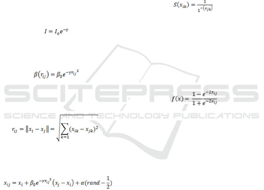
(2)

where I

is the original light intensity.

As a ﬁreﬂy’s attractiveness is proportional to the

light intensity seen by adjacent ﬁreﬂies, attractiveness

β of a ﬁreﬂy is now defined by

(3)

where β

is the attractiveness when distance

between the two fireflies, represented by r, is zero.

The distance between any two fireflies i and j is

the Cartesian distance:

(4)

where x

i,k

is the kth component of the spatial

coordinate x

of ith firefly.

The movement of a firefly i attracted to another

more attractive or brighter firefly j is determined by

(5)

where x

refers to the new value of the moved

firefly. The second term is for the attraction and the

third term is for the random movement using the

randomization parameter alpha α. The variable rand

is a random number generator uniformly distributed

in [0, 1].

In the study of Yang (2010), he was able to show

that the ﬁreﬂy algorithm performed more efficiently

and provided better success rate than PSO and GA.

This implies the very high potential of FA as a

powerful approach in solving NP-hard problems.

2.2.1 Modified Discrete Firefly Algorithm

The Modified Discrete Firefly Algorithm was studied

in 2011 by Pabrua (2011). The algorithm was derived

from the study of Sayadi et al. (2010). Pabrua (2011)

made discrete the modified firefly algorithm of

Sayadi et al. (2010) by applying the hyperbolic

tangent Sigmoid function (tanh), Equation 7, in

computing probabilities after the initialization of

fireflies and after every firefly movement. Sayadi et

al. (2010) used the following Sigmoid function to

replace the real number generated by the algorithm

with a binary number:

(6)

where x

is the calculated firefly movement from

firefly j to firefly k and S(x

) denotes the probability

of bit x

taking 1.

Although Sayadi et al. (2010) showed that the

modified Firefly algorithm is better than the existing

ant colony algorithm, Pabrua’s method of

discretization was still more effective (Pabrua, 2011).

The effectiveness of tanh in computing

probabilities is shown in Pabrua’s (2011) study

mentioning the data applied to generate or compare

the results:

(7)

where x

signifies the value of the movement of

firefly I towards firefly j.

2.3 Simulated Annealing

The name and principle of Simulated Annealing (SA)

algorithm is from the process of cooling molten metal.

If a metal cools rapidly, there is a limited time for its

atoms to settle into a tight lattice and are solidified in

a random configuration, which results in brittle

material. If the temperature is decreased very slowly,

the atoms are given enough time to settle into a strong

crystal (Luke, 2009).

SA starts with generating a new solution using the

objective or cost function given in the problem. The

probability that the new solution is accepted when the

following condition is true, otherwise, the current

configuration is used for the next steps (Kirkpatrick

et al., 1983):

(-ΔE/kT)

> rand (8)

where ΔE is the change of energy or the absolute

difference from the current solution to the new

solution function value. The Boltzmann constant is

represented by k, and the synthetic “temperature” is T.

The rand is the same in FA.

Hamdar (2008) used a starting temperature of

10,000, cooling rate of 0.9999, and absolute

temperature of 0.00001 as his parameters. Goossaert

(2010) solved TSP through SA with varying

parameters: a range of cooling rate from 0.95 to 0.99,

starting temperature range of 1e

+10

to 1e

+50

, and

ending temperature of 0.001 to 1. On the other hand,

Wright (2010) developed an automated parameter

selection for SA algorithm in which the best results

were obtained, thus this set of parameters were used

in this study.

2.4 Hybrid Algorithms

Over the years there has been a substantial amount of

progress on the fundamental ideas of designing

eﬃcient algorithms and the theoretical properties of

these methods of simulation. Each algorithm has

diﬀerent strengths and can be categorized by meeting

diﬀerent criteria based on the statistical properties of

the simulated Markov chain. It is therefore natural

that the question arises whether a better scheme can

be developed by combining the best aspects of

existing algorithms (Lee, 2011).

A hybrid algorithm can be designed from diﬀerent

perspectives by a variety of choices of algorithms to

combine and the way in which they are combined.

The primary motivation is to propose an eﬃcient

algorithm that overcomes identiﬁed weakness in the

individual algorithms.

Hybrid methods have previously been applied to

TSP. One of the hybrids solutions was developed by

Zarei and Meybodi (2002). Zarei and Meybodi used

both genetic algorithm (GA) and learning automata

(LA) simultaneously to search in state space. It has

been shown that the speed of finding answer increases

remarkably using LA and GA simultaneously in

search process, and it also prevents algorithm from

being trapped in local minima.

In this study, SA was used as a local optimizer of

the modified discrete firefly algorithm (MDFA). The

resulting hybrid algorithm was modified to address

the constraints of the garbage collection routing as a

TSP.

2.5 TSP Benchmark Datasets

Researchers of TSP have relied on the availability of

standard test instances to measure the efficiency of

the introduced solution methods. Since 1994, Gerhard

Reinelt have collected various TSP test instances

together with new examples drawn from industrial

applications and from geographic locations of cities

on maps. Reinelt’s library, called the TSPLIB,

contains over 100 examples with sizes from 14 cities

up to 85,900 cities. A few of these benchmark data

sets are PR152 (a 152-city problem), ST70 (a 70-city

problem), TS225 (225-city problem), and GR431

(431-city problem).

3 METHODOLOGY

The succeeding subsections present the proposed

algorithm utilizing a nature-inspired algorithm on an

optimization problem hybridized with a non-

population-based local heuristic method. The method

proposed is called Modified Discrete Firefly –

Simulated Annealing Algorithm (MDF-SA). The

Modified Discrete Firefly Algorithm is the main

algorithm throughout the procedure and is hybridized

with Simulated Annealing Algorithm as its local

optimizer. The subsections include details on

population initialization, local optimizer and

generation of a new solution. The performance

criteria to evaluate the results of the study is also

listed in this section as well as the benchmark data

sets used.

3.1 Benchmark Data Sets

The benchmark data sets downloaded from TSPLIB

used in this study are: PR152, ST70, TS225 and

GR431. These data sets were selected for their

similarity on their type of data inputs. The proposed

algorithm was also applied to the current garbage

collection routing system of the City of Davao. This

data set was taken from the Davao City Environment

and Natural Resource Office (CENRO). As seen in

Table 1, the city currently has 360 garbage collectors

distributed to 80 garbage trucks and collects an

average of 1,189 cubic meters of trash daily.

Garbage collection areas (areas the garbage truck

must visit) were represented by nodes m

p j

in a graph

and by data vectors z

upon implementation. Hence,

for each node, letting z

be a node and m

be the

distances between nodes, then

= (m

, m

, …, m

p j

)

where j is the jth node to be visited; and each

firefly (solution to the routing problem) from 1 to N

(total number of fireflies) is :

where V is the vth node to be visited.

3.2 Parameter Settings

The study adopted the parameters of Sayadi et al.

(2010) for MDFA while the parameters used in SA

algorithm was based on the method of Wright (2010)

as summarized in Table 2.

Table 2: Firefly algorithm (FA) and Simulated Annealing

(SA) parameters adopted from other studies.

Sayadi et al. (2010) Wright (2010)

FA Parameters Value SA Parameters Value

Attractiveness

(β

)

1.0 Initial

Temperature

(

initial

tem

)

50.00

Adaptable

Absorption

Coefficient (γ

)

0.8 Final

Temperature

(

inal_temp)

2.00

Random Step

size (α)

0.2 Geometric

Ratio (

)

0.99

Number of

fireflies (

)

30.0

Max number of

iterations

(

max

ite

)

50.0

3.3 Algorithms

MDFA by Pabrua (2011) is a modified version of the

DFA by Sayadi et al. (2010) wherein the Sigmoid

function is replaced with the hyperbolic tangent

sigmoid function. In this study, MDFA is made

hybrid with SA. Figure 1 shows the pseudocode of the

MDF-SA algorithm being proposed.

The algorithm begins with the initialization of the

algorithm parameters, namely N (number of fireflies),

gamma, beta_zero, alpha, and max_iter (Line 1). The

initialization of fireflies then follows (Line 2). Upon

the random generation, each firefly should produce

valid solutions.

The light intensity (I) of all fireflies is initialized

using the objective function (Line 3 to 5). The light

intensity in this context is defined as the sum of

the distances between cities in a specific order, solved

by Equation [2]. The firefly with the best light

intensity value, denoted as best is selected from the

randomly generated firefly population (Line 6). This

value is then initialized as the initial global best firefly

called global_best. For all fireflies, the light

intensities are compared and if the light intensity of

firefly j is less than the light intensity of firefly i, a

new position for firefly i is generated.

The generation of the new position is done in three

steps. First, is to compute the Euclidean distance

(Line 11) between firefly i and firefly j using equation

[4]. Second, is to compute the movement of firefly i

towards firefly j with the use of equation [5] (Line 13).

The third and final step of the position generation part

of the algorithm is to apply tanh (Equation [7]) to the

newly generated position so that these values are now

discretized, taking values in the range (-1, +1) (Line

14). The second and third are repeatedly iterated until

a valid solution is generated.

The next step of the algorithm is to convert the

positions of the firefly into a discrete matrix (Line 16),

wherein the lowest values in each row is assigned

with 1, while the others are assigned with the value 0.

A local search using SA is then employed to the

population of the fireflies (Line 19). The light

intensity of each firefly is updated after the

processing of the local search (Line 20). The values

for best and global_best are updated and the iteration

Initialize necessary parameters

Randomly generate initial

population of firefly F

’s

For each firefly

Calculate light intensity

End for

Select best and initialize as

global_best

for t = 1 to max_iter do

for i=1 to N

for j=1 to N, (i != j)

if light intensity j < light

intensity i

Calculate Euclidean distance

Calculate firefly movement

Apply tanh

while solution is not valid

Convert to discrete matrix

Subject moved firefly to SA

Update light intensity

End if

End for

Rank fireflies according to light

intensity

Update best and global_best

End for

Print/Report result to an output

module

Figure 1: Pseudocode of MDF-SA algorithm.

counter is incremented once (Line 23). It is then

checked if the number of iterations reached the

maximum number of iterations (max_iter). If the

maximum number of iteration is reached, then the

value of global_best is returned. Otherwise, the

execution of the algorithm continues.

3.3.1 Population Initialization

As discussed before, a firefly is a sequence of nodes.

The process of generating the population of the

fireflies is specified in the following discussion; the

pseudo code for population initialization is Figure 2.

Each firefly is initialized as a zero matrix. For all

initialized fireflies, a random permutation of the

given N nodes is generated and is designated to each.

For example, there are 50 fireflies and 70 visiting

nodes. Each firefly represents a unique solution. No

two fireflies shall correspond to the same solution.

The position of the node in the solution denotes its

priority in visitation. The node j assigned to visiting

priority n is assigned the value 1. This is true for all

nodes and all fireflies. Each value of the firefly

position is then restricted to a discrete value using the

hyperbolic tangent sigmoid function (Equation [7]).

3.3.2 Hyberbolic tangent sigmoid function

The effectiveness of tanh (Equation [7]) in computing

probabilities of placing a node in a visiting priority

was sused because of its superior results in the study

of Pabrua (2011).

In this study, the node j in visiting propriety k with

the lowest value is assigned to that priority denoted

by 1. Otherwise, the value of node j in visiting priority

k is not assigned to that priority and takes the value of

0. If the node with the minimum value has already

been assigned to a visiting priority, the next minimum

value is assigned to that specific priority.

Figure 2: Pseudo code for generating initial population of

fireflies.

3.3.3 Local Search - SA

In this study, simulated annealing (SA) was used as

the local search algorithm.

The first step of SA process is the initialization of

temperature (Line 1). The temperature is set in a

manner high enough to virtually accept all transitions

of solutions during the early stage of the process. The

moved firefly from the MDFA process is /initialized

as the current solution (Line 2). While the final

temperature has not yet been reached, a new solution

is then generated randomly in an attempt to replace

the current one, given the fact that it has a better

fitness value. The quantization error of the current

solution and the newly generated solution are

represented by evaluation (new) and evaluation

(current) (Line 5). If Edelta is less than zero or if a

randomly generated number from a uniform

Table 3: Summary of MDFA and MDF-SA results from four benchmarks.

Benchmark

Number of

Cities

MDFA MDF-SA Best Known

Solution

Best Solution Running

Time (ms)

Best Solution Running

Time (ms)

PR152

152 160980 279115 160980 278862 73682

ST70 70 3072 48366 1422 217647 675

TS225

225 277540 291067 277556 295731 126643

GR431

431 3519 666715 3518 676417 171414

1 for each firefly

2 Initialize as set of nodes

3 End for

4 for each firefly

5 for all nodes to be visited

6 do

7 do

8 Generate random number

(rand) between 1 to n

9 while rand is in permutation

list

10 while generated permutation

list already exists

11 End for

12 End for

13 for each firefly

14 for all nodes

15 Apply tanh

16 End for

17 Assign node visiting priority

18 End for

distribution [0, 1] is less than , the new

solution will replace the current solution (Lines 6 to

11). If the equilibrium condition is reached, the value

of the temperature is lowered by multiplying T to a

constant value k. This process is repeated until T

reaches a certain value, and the best solution is

returned.

3.3.4 Configuration of a New Solution

A swapping scheme was utilized in the configuration

of a new solution. To generate a new solution, two

nodes from the moved firefly is swapped. For an easy

understanding, an example is shown below:

Suppose a firefly F

has values:

= {D, A, C, B, W, M}

Upon random selection, nodes C and W are chosen.

These two nodes were then swapped resulting to:

= {D, A, W, B, C, M}

The swapping scheme in SA was applied until a

valid solution is found or until stopping criterion is

met.

3.4 Performance Criteria

Evaluation of the results of MDF-SA algorithm was

performed by:

a) Taking the average best solution quality and

corresponding running time for MDF-SA;

b) Taking the average best solution time among

the 30 runs for MDF-SA;

c) Taking the best solution quality and

corresponding running time among the 30

runs for the MDF-SA;

d) Taking the best solution time among the 30

runs for MDF-SA;

e) Running MDFA and getting the best

solution quality and its corresponding

running time among the 30 runs;

f) Comparing the best solution quality and

corresponding running time among the 30

runs for the MDF-SA to MDFA; and

g) Comparing the best solution quality for

MDF-SA to the current solid waste routing

system of Davao City.

The best solution quality refers to the smallest

value of the solution quality among the 30 runs. The

average best solution quality refers to the average of

the best solution quality of the 30 runs. The average

best solution time refers to the average of the running

time of the 30 runs.

The best running time indicated in this paper

refers to the best solution’s elapsed time in

milliseconds (ms) from the random initialization until

the best solution was found.

The better solution quality refers to the smaller

value of solution quality and better running time

refers to the smaller value on obtained running time.

3.5 Computer Specifications

The method proposed was implemented using Java

Programming language (JDK 1.6 and Netbeans IDE

v6.9.9 or above) because of its object-oriented

mechanism. Also, Java has built-in randomization

functions and data structures that are very usable in

the implementation phase. The program was run on

computer units which run on a Windows 7 operating

system o with a central processing unit of Intel®

Core™ i5-3380M Processor and 2GB RAM.

4 RESULTS AND DISCUSSION

In this chapter the evaluation of the performance of

MDF-SA algorithm is done in two sections, based on

the given 1) benchmark data sets, and 2) the real data

set, Davao City Solid Waste Collection Route.

4.1 Evaluation of the Performance of

the MDF-SA Algorithm

The results of MDF-SA algorithm is summarized in

Table 3. On applying the MDF-SA on PR152, among

the 30 runs, the best solution quality and best average

solution quality is 160980 units, which is

approximately 4327 units better than the average best

solution quality (165307.67 units). It took MDF-SA

Algorithm 278862 ms or approximately 4 minutes

and 38 seconds to obtain this solution.

The best solution time for MDF-SA algorithm run

for 276499 ms which is approximately 3291 ms faster

than the average running time (279790ms) of the 30

runs and 2362 ms faster than the running time of the

obtained solution quality. The best solution time

obtained a solution quality and average solution

quality of 167385 units.

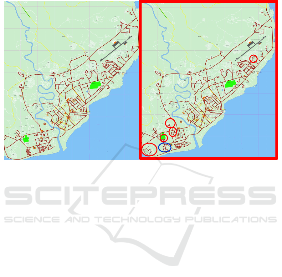
Figure 3: (A) Actual route of Davao City solid waste collection in Central Davao Area, (B) Route generated by MDF-SA.

On using ST70, the average best solution quality

of the 30 runs of using the ST70 data set is 1455.1

units. The best average solution quality is 1771 units.

The best solution quality is 1422 units with average

solution of 217647 units. From the start of the

execution of the algorithm, the solution gradually

converged to a lower value until the best solution was

obtained at the 50th iteration. It took MDF-SA

217647 ms to obtain the best solution quality.

The best solution time on using ST70 data set is

203399 ms, which is 11901ms faster than the average

running time (215301 ms) of the 30 runs and 57090

ms faster than the running time of the obtained best

solution quality among the 30 runs. The MDF-SA

execution with best solution time obtained the

solution quality and average solution quality of

167385 units.

In the use of TS225 data set, the average best

solution quality of the 30 runs 280439 units. The best

average solution is 277540 units, which is also the

best solution obtained among the 30 runs. It has a

running time of 293979 ms. The best solution time

among the 30 runs is 290903 ms which obtained a

best and average solution quality of 283540 units.

GR431 obtained the average best solution quality

of 3543.1 units. The best average solution quality

among the 30 runs is 3518 units with running time of

676417 ms. The best running time among the 30 runs

is 669816 ms with an obtained best and average

solution quality of 3542 units.

In using the Davao City Garbage Collection Data

Set, the best solution quality obtained is 731.2 km

with a running time of 497254ms. The average best

solution quality is 1144.5 km. The best average

solution quality among the 30 runs is also 731.2 km.

The fastest among the 30 runs is 481327 ms with best

and average solution quality of 1259.85 km.

4.2 Result for Davao City Garbage

Collection Data Set

Table 4 shows the best solutions obtained when

applying MDF-SA and MDFA algorithms to the

Davao City Garbage Collection data set. Based on the

results shown, MDF-SA obtained the best and

average solution of 731.2 km, and running time of

99450 ms. On the other hand, MDFA obtained the

best solution quality and best average solution quality,

both having values of 737.1 km and running time of

100937 ms.

The application of MDF-SA Algorithm to the

current garbage collection routing system of Davao

city resulted to a relative difference of 27.92% while

the application of MDFA to the same data set resulted

to relative difference of 28.95% from the current

routing distance.

It is observed that there is no significant difference

between the performance of the MDFA and MDF-SA

in terms of solution quality. In terms of running time

of the runs resulting to the best solution quality,

MDF-SA performed better than MDFA.

Table 4: Results of the application of MDF-SA Algorithm

and MDFA Algorithm to the Garbage Collection Routing

System of Davao City.

MDF-SA MDFA

Current

Routin

Best Solution

(km)

731.2 737.1 571.6*

Average Solution

(km)

731.2 737.1 -

Running Time

(

)

99450 100937 -

*manually calculated

Table 5: Summary of results of using MDF-SA and MDFA

to ST70, PR152, TS225, GR431 and Davao City solid

waste collection route.

Data Se

orithm with better Results

ST70 MDF-SA

PR152 MDF-SA and MDFA

TS225 MDFA

GR431 MDF-SA

Davao City Solid

Waste Collection

MDF-SA

When MDF-SA algorithm was applied to the

current Davao City Garbage collection route system,

it produced a better solution than the one generated

by MDFA. A summary of results using both

algorithms is summarized in Table 5. Factors causing

these differences in the performance of the hybrid

algorithm may have been the parameters of the

algorithm used and the approximation of the distances

among the nodes/garbage collection areas. Figure 3

shows the route generated by MDF-SA in comparison

with the actual route of the Davao City Solid Waste

Collection.

5 SUMMARY AND

CONCLUSIONS

This study hybridized the Discrete Firefly Algorithm

with Simulated Annealing

This study used tanh on Discrete Firefly

Algorithm (DFA) and hybridized it with Simulated

Annealing on discretizing the data to solve the NP-

complete problem specifically the travelling

salesman problem.

The researcher evaluated the performance of

MDF-SA Algorithm in five benchmarks: ST70,

PR152, TS225, GR431 and the current Davao City

Garbage Collection route. In using the MDF-SA

Algorithm and MDFA Algorithm, the researcher used

30 fireflies, 50 iterations, 0.8 gamma value, 1 initial

beta value, and 0.2 alpha value. On the hybridized

MDF-SA, the researcher used an initial temperature

of 50, final temperature of 2 and geometric ration of

0.99.

Both algorithms used the same parameters with

those in Sayadi et al. (2010) for the Firefly Algorithm

and Wright (2010) for the Simulated Annealing

parameters automation.

In terms of best solution quality, MDF-SA did not

improve the best known solution for all data sets.

MDF-SA and MDFA performed almost equally on 2

of the data sets: PR152 and GR431. MDFA

performed better by .01% relative error on one of the

data sets, TS225. MDF-SA performed much better on

the remaining 2 data sets: ST70 and the actual solid

waste collection system of Davao City.

In terms of running time, MDFA performed faster

on three of the data sets (ST70, TS225 and GR431)

compared to MDF-SA, which may have executed

REFERENCES

Agha, S.R. 2006. Optimizing Routing of Municipal Solid.
6 September 2012.
Awad, A.R., M.T. Aboul-Ela and R. Abu-Hassan. 2001.
Development of a Simplified Procedure for Routing
Solid Waste Collection. Scientia Iranica Publication. 6
September 2012. <http://www.scientiairanica.com/
PDF/ Articles/00000409/SI080109.pdf>.
Belien, J., Boeck, L. D., and J. V. Ackere. 2011. Municipal
Solid Waste Collection Problems:A Literature Review.
Hub Research Papers.
Bookstaber, D. 1997. Simulated Annealing for Traveling
Salesman Problem. 11 September 2011. <http://
www.eit.1th.se/fileadmin/eit/courses/ets061/Material/2
012/SATSP.pdf>.
Caliper Corporation. 2008. Automated Routing for Solid
Waste Collection Software. 6 September 2012.
<http://www.caliper.com/Press/pr990722 htm>.
Carillo, C. A. 2016, February 15. Waste management-
compliant Davao City struggles with garbage
segregation. Business World Online. Retrieved
December 15, 2016, from http://www.bworldonline
.com/content. php?section=Nation&title=waste-
management-compliant-davao-city-struggles-with-
garbage-segregation& id=123051
City of Davao. 2011a. Davao City - Geographical Location.
11 September 2012. <http://www.davaocity.gov.ph/
davao/ profile.aspx?id=location>.
City of Davao. 2011b. Demography – Environment. 2011.
davao/ demoenv.aspx>.
Dantzig, G., R. Fulkerson, and S. Johnson. 1954. Solution
of a large-scale traveling-salesman problem. Journal of
the Operations Research Society of America. 2.4:393-
410.
Dasgupta, S., C.H. Papadimitriou and U.V. Vazirani. 2006.
Chapter 8: NP-complete Problems. 7 September 2012.
<http://www.cs.berkeley.edu/~vazirani/algorithms/cha
p8.pdf>.
Goossaert, E. 2010. Simulated annealing applied to the
traveling salesman problem. 10 September 2010.
<http://codecapsule.com/2010/04/06/simulated-
annealing-traveling-salesman/>.
Goyal, S. 2010. A Survey on Travelling Salesman Problem.
11 September 2012 <http://www.cs.uwec.edu/MICS/
papers/mics2010_submission_51.pdf>.
Grom A. 2010. What is an NP-complete problem? 7
September 2012.
<http://stackoverflow.com/questions/210829/ what-is-
an-np-complete-problem>.
Hamdar, A. 2008. Simulated Annealing - Solving the
Travelling Salesman Problem (TSP). 7 September 2012.
<http://www.codeproject.com/Articles/26758/Simulat
ed-Annealing-Solving-the-Travelling-Salesma>.
Held M. and R. M. Karp. 1970. The traveling salesman
problem and minimum spanning trees. Operations
Research. 18.6:1132-1162.
Jensen, F. R. 2010. Using the Traveling Salesman Problem
in Bioinformatic Algorithms. 7 September 2012.
<http://www.daimi.au.dk/~cstorm/students/Rosenbech
Jensen_Dec2010.pdf>.
Kann, V. 2000. NPO Problems: Definitions and
Preliminaries. 7 September 2012. <http://www nada
kth.s/~viggo/ wwwcompendium/node2 html>.
Karadimas N.V., Papatzelou K., and V.G. Loumos. 2007.
Genetic Algorithms for Municipal Solid Waste
Collection and Routing Optimization. In: Boukis C.,
Pnevmatikakis A., Polymenakos L. (eds) Artificial
Intelligence and Innovations 2007: from Theory to
Applications. AIAI 2007. IFIP The International
Federation for Information Processing, vol 247.
Springer, Boston, MA.
Kirkpatrick S., C.D. Gelatt Jr., and M.P. Vecchi. 1983.
Optimization by simulated annealing. Science.
220.4598:671-680.
Lee, J. 2011. Issues in designing hybrid algorithms. 7
August 2012. <http://arxiv.org/pdf/1111.2609v1.pdf>.
Letchford, A. N. 2010. The Traveling Salesman Problem.
11 September 2011. <http://www.lancs.ac.uk/staff/
letchfoa/talks/TSP.pdf>.
Lin, S. 1965. Computer Solutions of the Traveling
Salesman Problem. 7 September 2012.
<http://www.alcatel-lucent.com/bstj/vol44-
1965/articles/bstj44-10-2245.pdf>.
Little, J.D.C., K. G. Murty, D. W. Sweeney, and C. Karel.
1963. An algorithm for the traveling salesman problem.
Operations Research. 11.6:972-989.
Luke, S. 2009. Essentials of Metaheuristics. Version 1.3. 7
August 2012. <http://cs.gu.edu/~sean/book/
metaheuristics/Essentials.pdf>.