Multi-labelled Image Segmentation in Irregular, Weighted Networks:
A Spatial Autocorrelation Approach
Rapha
¨
el Cer
´
e and Franc¸ois Bavaud
Department of Geography and Sustainability, University of Lausanne, Switzerland
Keywords:
Free Energy, Image Segmentation, Iterative Clustering, K-means, Laplacian, Modularity, Multivariate
Features, Ncut, Soft Membership, Spatial Autocorrelation, Spatial Clustering.
Abstract:
Image segmentation and spatial clustering both face the same primary problem, namely to gather together
spatial entities which are both spatially close and similar regarding their features. The parallelism is partic-
ularly obvious in the case of irregular, weighted networks, where methods borrowed from spatial analysis
and general data analysis (soft K-means) may serve at segmenting images, as illustrated on four examples.
Our semi-supervised approach considers soft memberships (fuzzy clustering) and attempts to minimize a free
energy functional made of three ingredients : a within-cluster features dispersion (hard K-means), a network
partitioning objective (such as the Ncut or the modularity) and a regularizing entropic term, enabling an itera-
tive computation of the locally optimal soft clusters. In particular, the second functional enjoys many possible
formulations, arguably helpful in unifying various conceptualizations of space through the probabilistic selec-
tion of pairs of neighbours, as well as their relation to spatial autocorrelation (Moran’s I).
1 INTRODUCTION
Regional data analysis, as performed on geographic
information systems, deals with a notion of “where”
(the spatial disposition of regions), a notion of “what”
(the regional features), and a notion of “how much”
(the relative importance of regions, as given by their
surface or the population size). The data define a
marked, weighted network, generally irregular (think
e.g. of administrative units): weighted vertices rep-
resent the regions, weighted edges measure the prox-
imity between regions, on which uni- or multivariate
features (the marks) are defined.
Much the same can be said of an image made
of pixels, that is a collection of elements embed-
ded in a bidimensional layout. The regularity of the
setup (regular grid, uniform weights, binary regular
adjacencies) is exploited in most segmentation algo-
rithms, but the latter may become inadapted, pre-
cisely, under irregular situations, such as pixels of var-
ious sizes or importance, aggregated pixels, irregular
boundaries or connectivites, multi-layered or partially
missing data.
This paper proposes an iterative algorithm
for semi-supervised image segmentation, directly
adapted from regional clustering procedures in spatial
analysis, themselves originating in (non-marked) net-
work clustering. In a nutshell, the purely spatial stan-
dard procedures aimed at Ncut minimisation (Shi and
Malik, 2000; Grady and Schwartz, 2006) or modular-
ity maximization (Newman, 2006) are enriched with
a features dissimilarity term, central in the K-means
approach, and further regularized by an entropy term,
favoring the emergence of soft clusters, and allowing
a iterative computation of locally optimal solutions.
The fields of spatial analysis, in particular spa-
tial clustering, on one hand, and image segmentation
on the other hand, seem currently to be investigated
by distinct, non-overlapping communities. Yet, both
communities arguably share the same what-versus-
where-trading challenge, aimed at obtaining clusters
both homogeneous and connected.
In this work in progress, we first define the main
quantities of interest and the iterative algorithm itself
(section 2). The definition of the canonical measure of
image homogeneity, namely Moran’s I in the present
spatial context, is recalled in section 2.3. Section (3)
illustrates the method on four case sudies. A conclu-
sion (section 4) lists some further research lines, to be
investigated in a close future. The appendix details
the construction of the so-called exchange matrix, as
well as the test of spatial autocorrelation in a weighted
setting.
62
Ceré, R. and Bavaud, F.
Multi-labelled Image Segmentation in Irregular, Weighted Networks: A Spatial Autocorrelation Approach.
DOI: 10.5220/0006322800620069
In Proceedings of the 3rd International Conference on Geographical Information Systems Theor y, Applications and Management (GISTAM 2017), pages 62-69
ISBN: 978-989-758-252-3
Copyright © 2017 by SCITEPRESS – Science and Technology Publications, Lda. All rights reserved

2 DEFINITIONS AND
FORMALISM
The formalism we consider extends the spatial au-
tocorrelation formalism used in Quantitative Geogra-
phy and Spatial Econometrics to the case of weighted,
irregular regions, as well as to multivariate features.
It turns out to be broad enough to provide a flexible
framework for unsupervised or semi-supervised gen-
eralized image segmentation, where the ”generalized
images” under consideration can be made of irregular
pixels, irregularly inter-connected, and endowed with
multivariate numerical features.
Space as a weighted network: the exchange matrix E
Specifically, consider n regions (generalized pix-
els) with relative weights f
i
> 0, summing to f
•
=
∑
n
i=1
f
i
= 1, together with an n ×n symmetric non-
negative exchange matrix E = (e
i j
), and weight-
compatible in the sense e
i•
=
∑
n
j=1
e
i j
= f
i
. The
exchange matrix E interprets as a joint probability
p(i, j) = e
i j
to select the pair of regions i and j
(edges), and defines a weighted unoriented network.
Its margins interpret as the probability p(i) = f
i
to se-
lect region i (vertices).
Weight-compatible exchange matrices E define a
continuous neighborhood relation between regions.
They can be constructed from f and the adja-
cency matrix A, or from another spatial proximity
of distance matrix (see the appendix). The row-
standardized matrix of spatial weights W = (w
i j
) of
spatial autoregressive models obtains as w
i j
= e
i j
/ f
i
,
and constitutes the transition matrix of a Markov
chain with stationary distribution f .
Multivariate features: the dissimilarity matrix D
Regional features can consist of univariate grey
levels, multivariate color or spectral intensities, or
(in a geographical context) any regional variable such
as the proportions of specific land uses, population
density, proportion of party B voters, etc. Multivari-
ate characteristics x
i
are suitably combined into n ×n
squared Euclidean dissimilarities D
i j
= kx
i
−x
j
k
2
.
2.1 Image Segmentation (Regional
Clustering)
A soft regional clustering or image segmentation into
m groups is described by non-negative n ×m mem-
bership matrix Z = (z
ig
) with z
ig
= p(g|i) denotes
the probability that region (pixel) i belongs to group
g, and obeys z
i•
=
∑
m
g=1
z
ig
= 1. The weights ρ of
the corresponding groups obtain as ρ
g
=
∑
i
f
i
z
ig
, and
the regional distribution of groups as f
g
i
= f
i
z
ig
/ρ
g
=
p(g|i), obeying f
g
•
= 1. The region-group dependency
can be measured by the mutual information
K [Z] =
∑
ig
p(i,g)ln
p(i,g)
p(i)p(g)
=
∑
ig
f
i
z
ig
ln
z
ig
ρ
g
(1)
A good clustering should consist of homogeneous
groups made of regions not too dissimilar regard-
ing their features, that is insuring a low value of the
within-group inertia (Bavaud, 2009)
∆
W
[Z] =
m
∑
g=1
ρ
g
∆
g
where ∆
g
=
1
2
∑
i j
f
g
i
f
g
j
D
i j
(2)
A good clustering should also avoid to separate a pair
of spatially strongly connected regions, that is to in-
sure a low value of the generalized cut
G[Z] =
1
2
∑
g
G(ρ
g
)
∑
i j
e
i j
(z
ig
−z
jg
)
2
(3)
where G(ρ) ≥ 0 is non-increasing in ρ. The choice
G(ρ) = 1/ρ amounts to the N-cut (Shi and Malik,
2000), while the choice G(ρ) = 1, we shall adopt
here, is equivalent to the modularity criterium (New-
man, 2006).
We consider the regularized clustering problem,
consisting in finding a clustering Z minimizing the
free energy functional
F [Z] = β∆
W
[Z] +
α
2
G[Z] + K [Z] (4)
The terms ∆
W
, respectively G , behaves as a features
dissimilarity energy, respectively a spatial energy, fa-
voring hard partitions obeying z
ig
= 0 or z
ig
= 1.
By contrast, the regularizing entropy term K favors
the emergence of soft clusterings. Setting α = 0
yields the soft K-means algorithm (Gaussian mix-
tures), where β is an inverse (dissimilarity) temper-
ature. Canceling the first-order derivative of the free
energy with respect to z
ig
under the constraints z
i•
= 1
yields the minimization condition
z
ig
=
ρ
g
exp(−βD
g
i
−α(Lz
g
)
i
)
∑
h
ρ
h
exp(−βD
h
i
−α(Lz
h
)
i
)
(5)
where D
g
i
=
∑
j
f
g
i
D
i j
−∆
g
is the squared Euclidean
dissimilarity from i to the centroid of group g, and
(Lz
g
)
i
= z
ig
−
∑
k
w
ik
z
kg
is the Laplacian of z
g
at i,
comparing its value to the average value of its neigh-
bourgs.
Multi-labelled Image Segmentation in Irregular, Weighted Networks: A Spatial Autocorrelation Approach
63

2.2 Iterative Procedure
Equation (5) can be solved iteratively, updating ρ
g
,
D
ig
and Lz
g
at each step, and converges towards a
local minimum Z
∞
of F [Z], which constitutes the
searched for soft spatial partition or image segmen-
tation. Z
∞
can be further hardened by assigning i to
group g = argmax
h
z
∞
ih
.
A semi-supervised implementation of the proce-
dure, imposing the membership of a few pixels (and
possibly breaking down the monotonic decrease of
F [Z]: see figure 5) goes as follow: first, the set Ω
of the n regions is partitioned into two disjoint, non-
empty sets, namely the user-defined tagged regions T,
and the free regions F, with Ω = T ∪F and T ∩F =
/
0.
The tagged set T itself consists of m non-empty dis-
joint subregions T = ∪
m
τ=1
T
τ
initially tagged with m
distinct strokes applied on a small number of pix-
els: they form the seeds of the g = 1, . . . , m figures
to be extracted, while the remaining regions will be
assigned to the background numbered g = 0.
Memberships Z = (z
ig
) consist of n ×(m+1) non-
negative matrices obeying
∑
m
g=0
z
ig
= 1. Their initial
value Z
0
is set as
z
0
ig





= 1 if i ∈ F and g = 0
= 1 if i ∈ T
τ
and g = τ
= 0 otherwise .
(6)
Iteration (5) is then performed. At the end of each
loop, the tagged regions are reset to their initial values
z
0
iτ
= 1 for all i ∈ T
τ
. After convergence, one expects
the hardened clusters obtained by assigning i to group
g = argmax
m
h=0
z
∞
ih
to consist of m connected figures
g = 1,...m each containing the tagged set T
g
, as well
as a remaining background supported on F.
The iterative image segmentation algorithm sum-
marized below (table 1) requires
1) a vector of n weights f
i
> 0 associated to each
pixel or region
2) a vector of n grey levels or multivariate character-
istics x
i
3) a n ×n binary, symmetric, off-diagonal adjacency
matrix A .
Retaining the soft memberships Z
(∞)
after conver-
gence could possibly provide a novel edge detection
mechanism (figure 5(b)), to be investigated in a
subsequent work. Namely, one expects z
(∞)
ig
= 0
or z
(∞)
ig
= 1 for pixels i located within the interior
of homogeneous groups, while 0 < z
(∞)
ig
< 1 for
pixels i located at the boundary of two of more
groups. As a consequence, the value of the entropy
Table 1: Summary of the iterative algorithm.
Begin
Compute the weight vector f ( f
i
= 1/n for regular grids)
Compute the binary adjacency matrix A
For given t > 0, compute the weight-compatible exchange matrix
E( f ,A,t) by (9), and the matrix of spatial weights as w
i j
= e
i j
/ f
i
Compute the features dissimilarity matrix D
i j
= kx
i
−x
j
k
2
Initialize the n ×(m + 1) membership matrix Z
0
as:
z
0
ig
= 1 if i ∈F and g = 0
z
0
ig)
= 1 if i ∈T
τ
and g = τ
z
0
ig
= 0 otherwise.
Loop : Z
(r+1)
for the r-th iteration, stop after convergence
Group weight : ρ
g
:=
∑
i
f
i
z
ig
Emission probabilities f
g
i
:=
f
i
z
ig
ρ
g
Dissimilarity to the centroid : D
g
i
:=
∑
j
f
g
j
D
i j
−∆
g
Laplacian: (Lz
g
)
i
= z
ig
−
∑
j
w
i j
z
jg
Compute z
(r+1)
ig
by (5)
Re-initialize z
(r+1)
ig
= δ
gτ
for i ∈T
τ
Attribute i ∈F to the group g = argmax
m
h=0
z
(∞)
ih
End
H
i
= −
∑
g
z
(∞)
ig
lnz
(∞)
ig
is presumably large for i located
at the group frontiers.
Deterministic profiling
The above iterative algorithm has been developed
with Python 2.7.12 (van Rossum, 1995) and per-
formed on a CPU Intel Core i7 two Core with a fre-
quency 3.1GHz (Mac OS X 10.10.5). Figure 1 sum-
marizes the “plain” computational performances (i.e.
without further optimizing such as Parallel computing
or Analysis of complexity) for the main ingredients at
stake, as a function of the number of pixels n in a reg-
ular setting.
2.3 Spatial Autocorrelation: Moran’s I
Average multivariate dissimilarities between regions
are expressed by inertias, generalizing the univariate
variances. The inertia between randomly selected re-
gions, and the local inertia between neighbours, are
respectively defined as
∆ :=
1
2
n
∑
i, j=1
f
i
f
j
D
i j
∆
loc
:=
1
2
n
∑
i, j=1
e
i j
D
i j
(7)
Comparing the global versus local inertias provides a
multivariate generalization of Moran’s I, namely,
I :=
∆ − ∆
loc
∆
(8)
whose values range in [−1,1]. A large positive I
is expected for an image made of large patchs char-
acterized with constant features, or at least varying
smoothly on average (spatial continuity = positive au-
tocorrelation). A large negative I characterizes an im-
age whose pixel features are contrasted, opposite to
GISTAM 2017 - 3rd International Conference on Geographical Information Systems Theory, Applications and Management
64

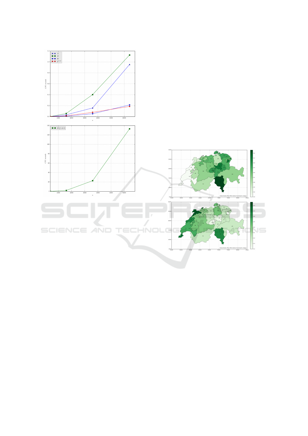
(a)
(b)
Figure 1: CPU times for a range of n ∈ [400,10000] pix-
els. (a) Computing of the binary “rook” adjacency matrix A
(with the Scikit-learn package (Pedregosa et al., 2011)), the
squared Euclidean profiles dissimilarity D, the Markov tran-
sition matrix W (for E given), as well as one single iteration
Z
(r)
→ Z
(r+1)
of the membership matrix. (b) The compu-
tation of the exchange matrix E( f , A,t) by (9) involves a
time-consuming complete eigen-decomposition.
their neighbours - such as a chess board with “rook”
adjacency. See the appendix for testing the statistical
significance of I.
3 ILLUSTRATIONS
We consider four small datasets:
• Swiss votes, an irregular, bivariate vector image
defined by two votations results at the canton level
(figure 2 and 3)
• the Portrait, a regular, trivariate (levels of red
green blue) image (figure 4)
• the Geometer, a regular, univariate (grey levels)
image (figure 5)
• Thun, a geographical univariate image depicting
the building density at the hectometre scale (cen-
sus blocks) in the region of Thun, Switzerland
(figure 6).
We first study the segmentation procedure, before
turing to spatial autocorrelation.
Figure 2 depicts the proportion of “yes” x
i
, respec-
tively y
i
, for each canton i (n = 26) for two emblem-
atic swiss popular initiatives, namely (a) the Initiative
against mass immigration which was accepted Febru-
ary the 9th, 2014, on the tie (50.3% of the citizen,
and the majority of cantons), respectively (b) the Ini-
tiative for minimum wages which was widely refused
May the 25, 2014 (23.7% of the citizens, and the ma-
jority of cantons). Both results have been aggregated
into the dissimilarity D
i j
= (x
i
−x
j
)
2
+(y
i
−y
j
)
2
, fur-
ther rescaled in the range [0,1]. Non-uniform canton
weights are defined relatively to the population 2015
density as f
i
= POP
i
/POP
total
, and the “queen” adja-
cency scheme has been adopted.
(a)
(b)
Figure 2: Swiss votes: percentage of “yes” for (a) the Initia-
tive against mass immigration and for (b) the Initiative for
minimum wages, at the canton level. ZH: Z
¨
urich, BE: Bern,
LU: Luzern, UR: Uri, SZ: Schwyz, OW: Obwalden, NW:
Nidwalden, GL: Glarus, ZG: Zug, FR: Fribourg/Freibourg,
SO: Solothurn, BS: Basel-Stadt, BL: Basel-Landschaft, SH:
Schaffhausen, AR: Appenzell-Aus., AI: Appenzell-Inn.,
SG: St. Gallen, GR: Grischun, AG: Aargau, TG: Thurgau,
TI: Ticino, VD: Vaud, VS: Valais/Wallis, NE: Neuch
ˆ
atel,
GE: Gen
`
eve, JU: Jura.
Figure 4 depicts a regular multivariate image
(RGB) of size 50 ×54 with uniform weight vector
f
i
= 1/n for n = 2700. Also, the binary adjacency
matrix has been built under the “queen” scheme (8
neighbourghs), and D
i j
is the sum of the squared dif-
ferences between color intensities.
Segmentation evaluation
The silhouette coefficient s ∈ [−1, 1] is a mea-
sure of the tightness and separation associated to a
dissimilarity-based clustering, and defines as s = (b−
a)/max(a,b) ∈ [−1,1], where a is the mean intra-
Multi-labelled Image Segmentation in Irregular, Weighted Networks: A Spatial Autocorrelation Approach
65

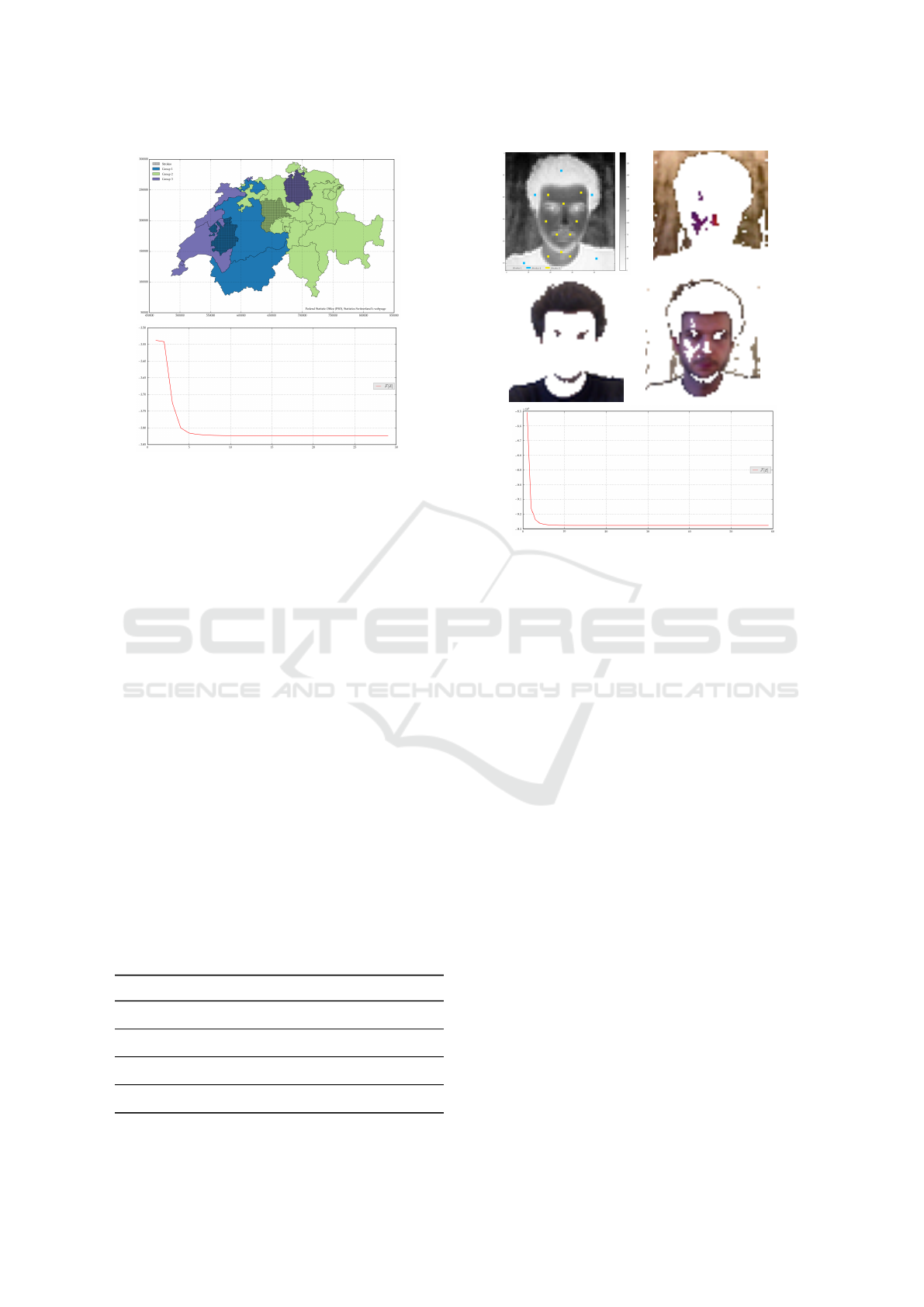
(a)
(b)
Figure 3: Swiss votes, continued: (a) hard assignment i to
group g obtained from the intial strokes FR ∈ Group 1, LU
∈ Group 2 and ZH ∈ Group 3 after 29 iterations, with β =
1/0.007 and α = 0.7143. (b) depicts the decrease of the free
energy functional F [Z] during the iteration.
cluster dissimilarity, and b the mean “nearest-cluster”
dissimilarity (Rousseeuw, 1987).
Table 2 gives the silhouette coefficients s for three
groups (including the background group) under four
segmentation algorithms, possibly converted to hard
clustering after convergence, namely: hard K-means
with random initialization of centroids, EM Gaussian
Mixture modeling with diagonal covariance matrix
(Pedregosa et al., 2011), our own iterative clustering
algorithm (table 1) with α = 0 and β optimized so as
to maximize s, and finally the iterative clustering al-
gorithm (table 1) with the same value of β, but with
α = 1 in order to take into account the spatial contri-
bution Lz
g
. Spatial autocorrelation
Table 2: Segmentation evaluation : silhouette coefficients
s under four datasets and four clustering algorithms (see
text). The iterative algorithm with α = 0 yields the opti-
mal values β
0
= 1/0.0052 (Swiss votes), β
0
= 1/0.0052
(Portrait), β
0
= 1/0.00342 (Geometer) and β
0
= 1/0.0052
(Thun), and should be equivalent to the EM algorithm. The
lower performance of the iterative algorithm (table 1) for
the Swiss votes dataset is unexpected, and under current in-
vestigation.
Dataset m+1 s
K-means
s
EM
s
β
0
,α=0
s
β
0
,α=1
Swiss votes 3 0.41 0.40 0.28 0.28
Portrait 3 0.57 0.57 0.56 0.56
Geometer 3 0.66 0.63 0.64 0.65
Thun 3 0.77 0.70 0.76 0.77
(a) (b)
(c) (d)
Figure 4: the Portrait: (a) initial configuration (intensity of
red) and strokes (colored pixels); (b) hard assignment to
background group g = 0; (c) hard assignment to g = 1, and
(d) hard assignment to g = 2, obtained after 99 iterations,
with β = 1/0.001 and α = 1. Bottom: behavior of the free
energy functional during the iteration.
Figure 7 presents the values of Moran’s I (8), its
expectation and variance under the null hypothesis
of no autocorrelation, and its standardized z-value on
which the normal test is based (see the appendix), for
a diffusion time t = 1.
Figures 8, 9, 10 and 11 depict, for varying t, the
values of Moran’s I and its expectation E
0
(I) (top),
its variance Var
0
(I) (middle) and its standardized z
normal test value (bottom) for the four illustrations
under consideration.
The freely adjustable parameter t controls the
neighbors range of the diffusive Markov diffusion
process W (t), and the behaviour of the plotted quan-
tities relatively to t should presumably reflect the size
of patches consisting of similar pixels.
4 DISCUSSION
The present study constitutes a first attempt aimed to
unify two little interacting domains – image segmen-
tation and regional clustering – yet arguably very sim-
ilar in their aims, and both relevant to spatial anal-
ysis. Spatial autocorrelation, in its general formula-
tion (irregular, weighted networks) emerges as a com-
mon unifying paradigm, worth extending in the future
GISTAM 2017 - 3rd International Conference on Geographical Information Systems Theory, Applications and Management
66

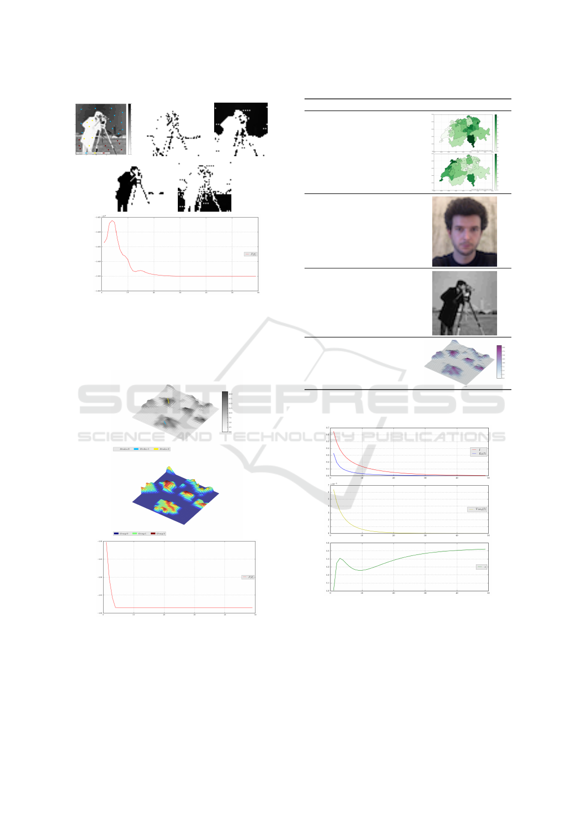
(a) (b) (c)
(d) (e)
Figure 5: the Geometer: (a) raster univariate image (grey
levels x
i
range in the interval [0,255]) of size n = 50 ×50 =
2500 with initial strokes; (b) background group g = 0; (c)
g = 1; (d) g = 2, and (e) g = 3, obtained after 60 iterations,
with parameters β = 1/0.003 and α = 0.017. Bottom: be-
havior of the free energy functional during the iteration, ini-
tially increasing.
Figure 6: Thun example. Top: raster univariate image of
size n = 20×24 = 480, depicting the the population density
per hectometer, rescaled in in the interval of [0,27]. Mid-
dle: groups g = 0 (blue, background), g = 1 (green) and
g = 2 (purple), obtained after 50 iterations, with parameters
β = 1/0.0003 and α = 0.17. Bottom: behavior of the free
energy.
I E
0
(I) Var
0
(I) z Image(s)
0.65 0.33 0.0064 4.01
0.23 0.10 2.15 ×10
−6
88.92
0.21 0.099 2.12 ×10
−6
74.41
0.69 0.40 0.0001 24.49
Figure 7: Moran’s I and standardized test value z for the
four illustrations.
Figure 8: Swiss votes: Moran’s I (top) and standardized z
normal test value (bottom) for t ∈ [1, 50].
to local indicators (LISA) (Anselin, 1995). The pro-
posed iterative approach can be considered as a gen-
eralization of the EM soft clustering for mixture mod-
els, containing an additional spatial term.
Alternative spatial or “Dirichlet-like” function-
als G[Z], such as the N-cut specification mentioned
in section (2), or “p-Laplacians” (Bougleux et al.,
Multi-labelled Image Segmentation in Irregular, Weighted Networks: A Spatial Autocorrelation Approach
67

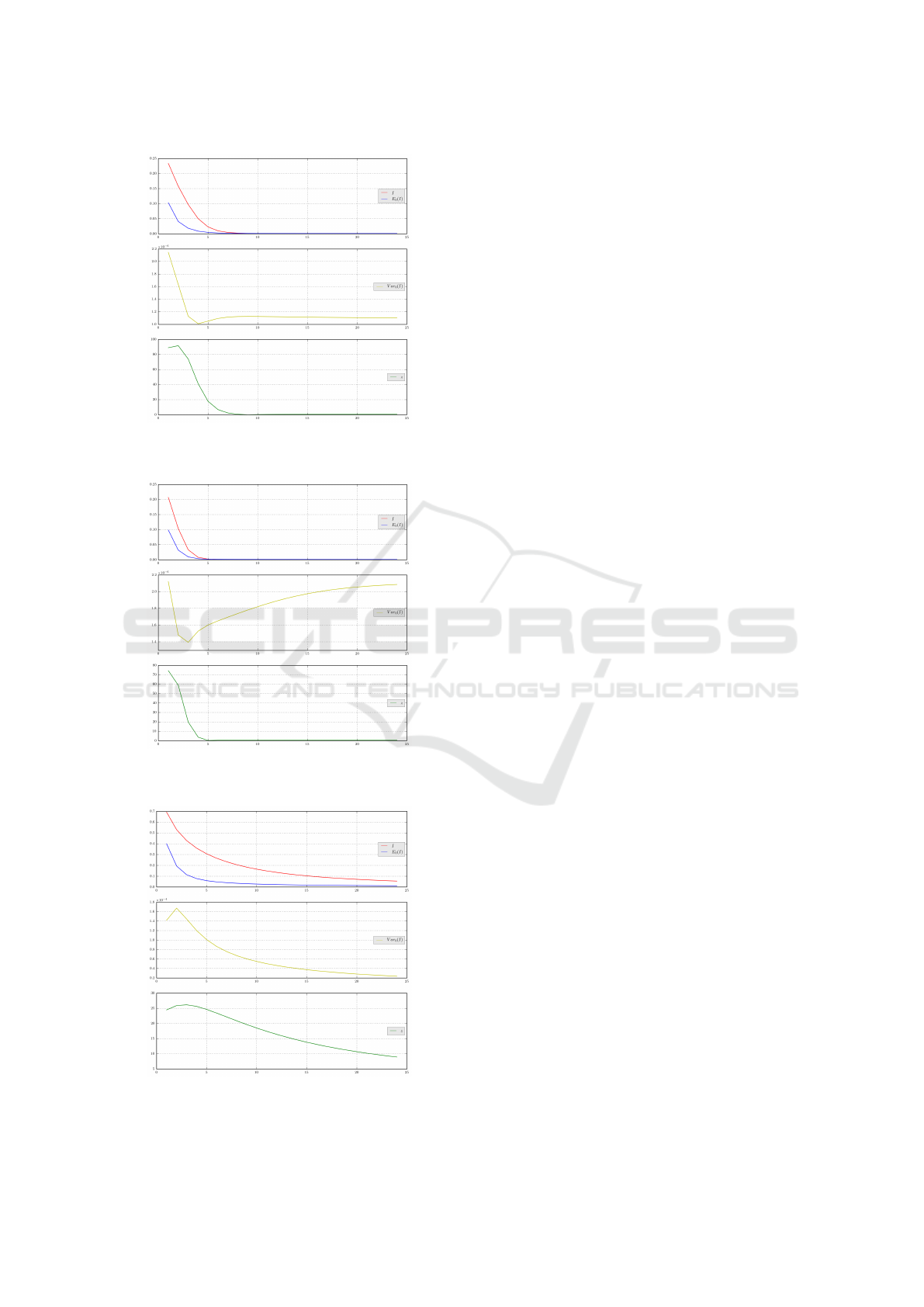
Figure 9: the Portait: Moran’s I (top) and standardized z
normal test value (bottom) for t ∈ [1, 25].
Figure 10: the Geometer: Moran’s I (top) and standardized
z normal test value (bottom) for t ∈ [1, 25].
Figure 11: Thun: Moran’s I (top) and standardized z normal
test value (bottom) for t ∈ [1, 25].
2009) should be considered, as is the relation to the
Mumford-Shah functional (Chambolle et al., 2012)
(Bar et al., 2011). Note that G[Z] can be adjusted
in two obvious, independent ways, namely by consid-
ering alternative weight-compatible specifications to
E(A, f ), and by considering alternative forms G(ρ) in
(3).
Besides those energy-based approaches, the en-
tropic part K [Z] can be introduced as a simple reg-
ularization term, or, as in the EM soft clustering,
as originating from maximizing the log-likelihood of
a statistical model (MAP approach), as in (Besag,
1986) or (Greig et al., 1989); see also (Couprie et al.,
2011). Probabilistic formulations of the image seg-
mentation problem should, as attested from spatial au-
tocorrelation studies, benefit from results and experi-
ence in model-based clustering and latent modeling.
Alternatively, the virtue of random walk ap-
proaches, intimately connected to Markov chains and
weighted networks, electric of not, has been attested
in semi-supervised clustering in general, and image
segmentation in particular (Grady, 2006). One key
quantity is the probability that a random walk starting
from a free pixel reaches first each of the m tagged
regions – a problem well-known to be related to the
Dirichlet differential problem with suitable boundary
conditions, and to the computation of electric poten-
tials (Doyle and Snell, 1984).
Yet, in the probabilistic formulations of the multi-
source, multi-target random walks (Guex, 2016),
the capacities and the edge resistances turn out to
be freely, separately adjustable (Bavaud and Guex,
2012). In the image segmentation context, it is tempt-
ing to identify the capacity contribution as a spatial
term enabling transitions between neighbors, and the
resistance contribution as a barrier preventing transi-
tions between too dissimilar pixels; to which extent
this line of research could prove itself innovative and
efficient should be addressed in a near future.
REFERENCES
Anselin, L. (1995). Local indicators of spatial association-
lisa. Geographical analysis, 27(2):93–115.
Bar, L., Chan, T. F., Chung, G., Jung, M., Kiryati, N.,
Mohieddine, R., Sochen, N., and Vese, L. A. (2011).
Mumford and shah model and its applications to im-
age segmentation and image restoration. In Handbook
of mathematical methods in imaging, pages 1095–
1157. Springer.
Bavaud, F. (2009). Aggregation invariance in general clus-
tering approaches. Advances in Data Analysis and
Classification, 3(3):205–225.
Bavaud, F. (2014). Spatial weights: constructing weight-
compatible exchange matrices from proximity matri-
GISTAM 2017 - 3rd International Conference on Geographical Information Systems Theory, Applications and Management
68

ces. In International Conference on Geographic In-
formation Science, pages 81–96. Springer.
Bavaud, F. and Guex, G. (2012). Interpolating between ran-
dom walks and shortest paths: a path functional ap-
proach. In International Conference on Social Infor-
matics, pages 68–81. Springer.
Besag, J. (1986). On the statistical analysis of dirty pic-
tures. Journal of the Royal Statistical Society. Series
B (Methodological), pages 259–302.
Bougleux, S., Elmoataz, A., and Melkemi, M. (2009). Lo-
cal and nonlocal discrete regularization on weighted
graphs for image and mesh processing. International
journal of computer vision, 84(2):220–236.
Chambolle, A., Cremers, D., and Pock, T. (2012). A con-
vex approach to minimal partitions. SIAM Journal on
Imaging Sciences, 5(4):1113–1158.
Couprie, C., Grady, L., Najman, L., and Talbot, H. (2011).
Power watershed: A unifying graph-based optimiza-
tion framework. IEEE Transactions on Pattern Anal-
ysis and Machine Intelligence, 33(7):1384–1399.
Doyle, P. G. and Snell, J. L. (1984). Random walks
and electric networks. Mathematical Association of
America,.
Grady, L. (2006). Random walks for image segmentation.
IEEE transactions on pattern analysis and machine
intelligence, 28(11):1768–1783.
Grady, L. and Schwartz, E. L. (2006). Isoperimetric graph
partitioning for image segmentation. IEEE transac-
tions on pattern analysis and machine intelligence,
28(3):469–475.
Greig, D. M., Porteous, B. T., and Seheult, A. H. (1989).
Exact maximum a posteriori estimation for binary im-
ages. Journal of the Royal Statistical Society. Series B
(Methodological), pages 271–279.
Guex, G. (2016). Interpolating between random walks
and optimal transportation routes: Flow with multiple
sources and targets. Physica A: Statistical Mechanics
and its Applications, 450:264–277.
Newman, M. E. J. (2006). Modularity and community
structure in networks. Proceedings of the National
Academy of Sciences, 103(23):8577–8582.
Pedregosa, F., Varoquaux, G., Gramfort, A., Michel, V.,
Thirion, B., Grisel, O., Blondel, M., Prettenhofer,
P., Weiss, R., Dubourg, V., Vanderplas, J., Passos,
A., Cournapeau, D., Brucher, M., Perrot, M., and
Duchesnay, E. (2011). Scikit-learn: Machine learning
in Python. Journal of Machine Learning Research,
12:2825–2830.
Rousseeuw, P. J. (1987). Silhouettes: A graphical aid to
the interpretation and validation of cluster analysis.
Journal of Computational and Applied Mathematics,
20:53–65.
Schneider, M. H. and Zenios, S. A. (1990). A comparative
study of algorithms for matrix balancing. Operations
research, 38(3):439–455.
Shi, J. and Malik, J. (2000). Normalized cuts and image
segmentation. IEEE Transactions on pattern analysis
and machine intelligence, 22(8):888–905.
van Rossum, G. (1995). Python tutorial. Technical Re-
port CS-R9526, Centrum voor Wiskunde en Informat-
ica (CWI), Amsterdam.
APPENDIX
Computing E(A, f )
Constructing an exchange matrix E (section 2)
both weight-compatible (that is obeying E1 = f ,
where the regional weights f are given) and reflecting
the spatial structure contained in the binary adjacency
matrix A = (a
i j
) is not trivial, nor that difficult either.
A natural attempt consists in determining a vector
c such that e
i j
= c
i
a
i j
c
j
. The problem can be essen-
tially solved by Sinkhorn iterative fitting (Schneider
and Zenios, 1990)
In this paper, we alternatively consider A as the
infinitesimal generator of a continuous Markov chain
at time t > 0, which yields the diffusive specification
(Bavaud, 2014)
E ≡ E(A, f ,t) = Π
1/2
exp(−tΨ) Π
1/2
(9)
where Π = diag( f ), and
Ψ = Π
−1/2
LA
trace(LA)
Π
−1/2
(LA)
i j
= δ
i j
a
i•
−a
i j
LA is the Laplacian of matrix A, and matrix exponen-
tiation (9) can be performed by spectral decomposi-
tion of Ψ.
The resulting E is semi-definite positive, with lim-
its E = Π for t → 0 (diagonal spatial weights W , ex-
pressing complete spatial autarchy), and E = f f
0
for
t → ∞ (constant spatial weights W , expressing com-
plete mobility). Identity trace(E(t)) = 1 −t + 0(t
2
)
(Bavaud, 2014) shows t to measure, for t  1, the
proportion of distinct regional pairs in the joint distri-
bution E.
Testing spatial autocorrelation
Under the null hypothesis H
0
of absence of spa-
tial autocorrelation, and under normal approximation,
the expected value of the multivariate Moran’s I reads
(Bavaud, 2014)
E
0
(I) =
tr(W ) −1
n −1
where w
i j
=
e
i j
f
i
and its the variance reads
Var
0
(I) =
2
n
2
−1

trace(W
2
) −1 −
(trace(W ) −1)
2
n −1

Spatial autocorrelation is thus significant at level α if
z := |I −E
0
(I)|/
√
Var
0
(I) ≥ u
1−
α
2
, where u
1−
α
2
is the
α
th
quantile of the standard normal distribution.
Multi-labelled Image Segmentation in Irregular, Weighted Networks: A Spatial Autocorrelation Approach
69