
Estimating Reference Evapotranspiration using Data Mining Prediction
Models and Feature Selection
Hinessa Dantas Caminha
1
, Ticiana Coelho da Silva
1
, Atslands Rego da Rocha
2
and S´ılvio Carlos R. Vieira Lima
3
1
Federal University of Cear´a, Campus de Quixad´a, Quixad´a, CE, Brazil
2
Federal University of Cear´a, Campus do Pici, Fortaleza, CE, Brazil
3
INOVAGRI Institute, Av. Santos Dumont 3131-A, Fortaleza, CE, Brazil
Keywords:
Data Mining, Irrigated Agriculture, M5P, Linear Regression.
Abstract:
Since the irrigated agriculture is the most water-consuming sector in Brazil, it is a challenge to use water
in a sustainable way. Evapotranspiration is the combination process of transferring moisture from the earth
to the atmosphere by evaporation and transpiration from plants. By estimating this rate of loss, farmers can
efficiently manage the crop water requirement and how much water is available. In this work, we propose
prediction models, which can estimate the evapotranspiration based on climatic data collected by an automatic
meteorological station. Climatic data are multidimensional, therefore by reducing the data dimensionality,
then irrelevant, redundant or non-significant data can be removed from the results. In this way, we consider in
the proposed solution to apply feature selection techniques before generating the prediction model. Thus, we
can estimate the reference evapotranspiration according to the collected climatic variables. The experiments
results concluded that models with high accuracy can be generated by M5’ algorithm with feature selection
techniques.
1 INTRODUCTION
Reducing poverty and the food insecurity are cru-
cial. Irrigated agriculture plays an important role in
this goal to be achieved, by ensuring innovative ap-
proaches that lead to increased productivity and pro-
vide sustainable solutions (fao, 2015). According to
(inf, 2015), irrigation is responsible for 72% of water
consumed in Brazil. While other sectors are expand-
ing such as water supply, industry, manufacturing and
the environment itself, the need for water resources
grows as well. Therefore, the agriculture sector must
be responsible for reviewing and adjusting its meth-
ods according to the amount of water available to use
(Garces-Restrepo et al., 2007).
Irrigation management aims at proposing tech-
niques to increase the water preservation and the en-
ergy resources without reducing the economic pro-
duction of the crop. This can be done based on how
much water is required to cultivate as well as the soil
characteristics and the soil capacity to retain water.
Among the several current techniques, we can men-
tion the technique of climate monitoring, which con-
sists of the use of weather stations to provide cli-
matic data and estimate the water consumption of
the crop. Such estimation is computed by using the
evapotranspiration concept. According to (Frizzone
et al., 2013), the evapotranspiration (ET) means the
simultaneous occurrence of evaporation and transpi-
ration on the vegetation. Its rate is usually described
in millimeters (mm) for a given unit of time (which
can be an hour, day, decade, month or even an entire
year) and it expresses the amount of water lost from a
cropped surface in units of water depth (Allen et al.,
1998). In order to compute the crop water require-
ment, which refers to the amount of water that needs
to be supplied, it is performed an estimation based on
the reference evapotranspiration (ET
0
) and the crop
coefficient (K
c
) (Frizzone et al., 2013). This approach
(K
c
x ET
0
) provides a simple, convenient and repro-
ducible way to estimate the evapotranspiration (ET)
from a variety of crops and climatic conditions (Allen
et al., 1998).
The only factors affecting ET
0
are climatic param-
eters. Consequently, ET
0
is a climatic parameter, and
it can be computed from the weather data. ET
0
ex-
presses the evaporating power of the atmosphere at a
particular location and time of the year and it does not
272
Caminha, H., Silva, T., Rocha, A. and Lima, S.
Estimating Reference Evapotranspiration using Data Mining Prediction Models and Feature Selection.
DOI: 10.5220/0006327202720279
In Proceedings of the 19th International Conference on Enterprise Information Systems (ICEIS 2017) - Volume 1, pages 272-279
ISBN: 978-989-758-247-9
Copyright © 2017 by SCITEPRESS – Science and Technology Publications, Lda. All rights reserved

consider the crop characteristics and soil factors. The
FAO Penman-Monteith method (Allen et al., 1998)
is recommended as the sole method for determining
ET
0
. However, their use is complex and requires that
all climate variables be present. In this way, several
procedures have been developed for estimating miss-
ing climatic parameters.
Climatic data can also be analyzed by data min-
ing techniques. Data mining refers to the applica-
tion of techniques and algorithms for recognizing pat-
terns and models about the data being able to gen-
erate knowledge. There exist several papers which
analyze meteorological and climatic data, such as
(Xavier et al., 2016), (Hendrawan and Murase, 2011),
(Rahimikhoob, 2014) and (Sawalkarand Dixit, 2015).
We aim to analyze these data as well by using data
mining. In this paper, we aim to answer the follow-
ing research question: Is it possible to estimate refer-
ence evapotranspiration without loss of accuracy re-
gardless of the availability of all variables? To solve
this problem, we use a dataset with historical series,
generated by a weather station in the UFC Quixad´a,
Cear´a, Brazil. The prediction models were created
by using the data mining technique M5’ proposed on
(Wang and Witten, 1996). M5’ created more than one
function to calculate the reference evapotranspiration,
and it specifically refers to the crops present in the
environments where the climatic data were collected.
Another example of such techniques to generate pre-
diction models is Regression, which learns a function
that maps a data item to a real-valued prediction vari-
able (Fayyad et al., 1996). In this work, we apply
linear regression models as well to estimate the refer-
ence evapotranspiration based on climatic data.
However, the data collected from weather stations
can be inaccurate or missing due to several reasons
such as sensor failure, calibration problems, wireless
transmission loss or environmental noise. Moreover,
we can also highlight the existence of missing val-
ues due to the problems with data storage or datalog-
ger power failures. In order to overcome these prob-
lems, feature selection techniques can help to handle
the fluctuating, inaccuracy or imprecision of the sen-
sor readings in a proper way and avoid that a wrong
decision would be made.
We may notice that related papers proposed mod-
els usually applied to calculate the reference evap-
otranspiration and the models are not composed of
all attributes of climatic data. Moreover, as climatic
data are multidimensional, by reducing the number
of attributes so that irrelevant, redundant or non-
significant data might be removed from results (Liu
and Yu, 2005), we can save computation time in the
analysis of these data as well.
Data pre-processing is a significant step in the
knowledge discovery process since quality decisions
must be based on quality data. The Feature Selection
is one of the data reduction techniques, which the goal
is to find a minimum set of attributes such that the re-
sulting probability distribution of the data classes is as
close as possible to the original distribution obtained
using all attributes (Karegowda et al., 2010).
In this way, we propose to apply feature selec-
tion before generating the prediction model for ref-
erence evapotranspiration (ET
0
). In this paper, the
model to predict the reference evapotranspiration was
generated by using the attributes selected. Our so-
lution generated two models, one by applying M5’
algorithm and another one by applying linear regres-
sion. We have performed many experiments in or-
der to compare the models generated with the origi-
nal data (without feature selection) and with feature
selection in order to discover which one results in a
more accurate model.
The remaining of this paper is structured as fol-
lows. Section 2 reports our solution and Section
3 presents the performed experiments. Section 4
presents the related works. Finally, Section 5, we
draw conclusions and propose future works.
2 METHODOLOGY
We aim at discovering a model to predict the ET
0
value for the collected data of a weather station. To
achieve this goal, we used an adaptation of the KDD
(standing for Knowledge Discovery in Databases)
process described in (Fayyad et al., 1996) to drive our
methodology. The next subsections correspond to the
steps of the process and how they were executed.
2.1 Data Collection
The first stage consists to collect climatic data gen-
erated by the weather station. They are related to the
climatic conditions monitored by the station in the pe-
riod from 16th of June to 19th of October of 2016 at
the city of Quixad´a, Cear´a, Brazil. The data collec-
tion were performed through a serial connection with
the data logger of the station provided by software
PC200W (pc2, 2016). The dataset was stored in CSV
files.
The original dataset contains 3191 numeric type
tuples, no missing values and it is composed of the
attributes described in Table 1.
Estimating Reference Evapotranspiration using Data Mining Prediction Models and Feature Selection
273
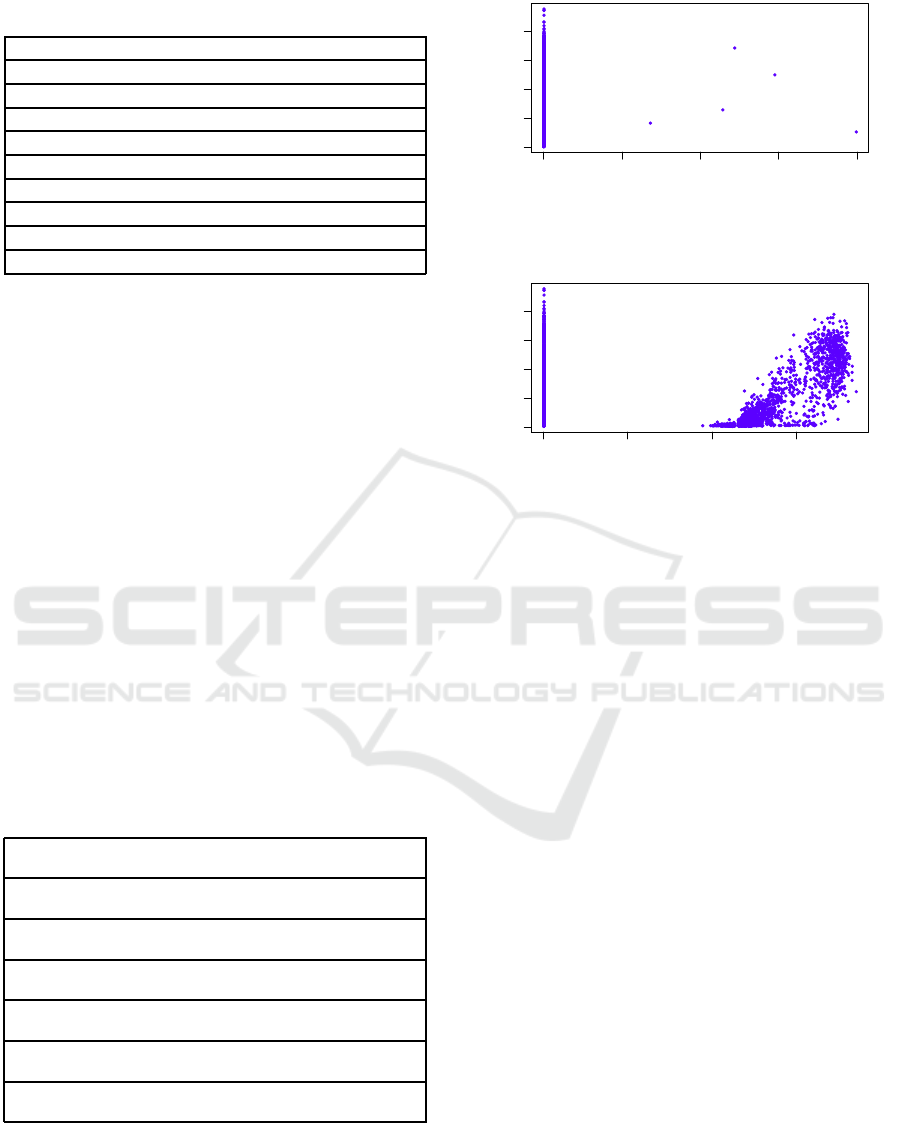
Table 1: Attributes present in the dataset.
Attributes
ET
0
Timestamp
Precipitation (mm)
Wind Speed
Solar radiation (total and average)
Temperature (maximum and minimum)
Relative air humidity (min, max and average)
Air temperature (min, max and average)
Atmospheric pressure (min, max and average)
2.2 Pre-processing
Data pre-processing refers to collecting, clean, and
persist the data in a file or table for future analysis.
In this step, the instances which have a non-standard
value for any of the attributes are removed from the
dataset. We call these instances outliers, and they can
affect the accuracy of the prediction model. In or-
der to discover the outliers, for each attribute of the
dataset, we studied how ET
0
varies with each attribute
presented in Table 1.
Figures 1 and 2 show the variation of the ET
0
value versus the average of solar radiation and the
maximum air temperature, respectively. By plotting,
we could find the outliers tuples that should be re-
moved from the dataset.
Based on our study, we remove the instances con-
taining the values presented in Table 2. After the data
pre-processing, the number of instances in the dataset
reduced to 1120.
Table 2: Removed instances.
Precipitation > 1 Maximum atmospheric pressure
> 625.000
Medium solar radiation >
25.4809
Total solar radiation > 6000000
Minimum temperature > 23.4105 Medium relative humidity >
99.8006
Wind speed > 4 Maximum temperature >
24.8820
Minimum air temperature < 1 Minimum air temperature >
36.692
Maximum air temperature < 1 Minimum air temperature >
37.965
Minimum relative air humidity >
87.062
Maximum relative air humidity >
95.5
2.3 Feature Selection
In this step, after the data pre-processing, the fea-
ture selection algorithms were performed. For this
0 5000 10000 15000 20000
0.00 0.10 0.20
Medium solar radiation
ET0
Figure 1: Variation of the medium solar radiation versus
ET
0
value.
0 10000 20000 30000
0.00 0.10 0.20
Maximum air temperature
ET0
Figure 2: Variation of the maximum air temperature versus
ET
0
value.
purpose, we use the WEKA framework (Hall et al.,
2009). The cross-validation method with ten folds
was used to define the training and test sets.
We experimented only the filter approach by ap-
plying the CFS algorithm (Hall, 2000). The CFS is
a simple filter algorithm that ranks feature subsets
according to a correlation based heuristic evaluation
function. The bias of the evaluationfunction is toward
subsets that contain features that are highly correlated
with the class and uncorrelated with each other. Ir-
relevant features should be ignored because they will
have low correlation with the class (Hall, 1999). We
evaluated all search algorithms present in WEKA and
that were compatible with CFS. However, the Best
First, Exhaustive Search Genetic Search, and Random
Search algorithms achieved the best accuracy when
generating the predictive models.
In Table 3, the correlation coefficients generated
by the models can be observed using the attributes se-
lected by each search algorithm. Table 4 shows which
attributes were selected by each algorithm.
2.4 Prediction Model
We created the prediction models by applying the
linear regression and M5P algorithms, both imple-
mented in the WEKA tool. In order to create the mod-
els, we split the dataset into 70% for training and 30%
for testing.
ICEIS 2017 - 19th International Conference on Enterprise Information Systems
274

Table 3: Correlation for the generated models by applying
different search algorithms.
Algorithm M5P Linear Regression
CFS + Greedy Stepwise 0.988 0.9511
CFS + Linear Forward 0.988 0.9511
CFS + Subset Size Forward Selection 0.988 0.9511
CFS + Scatter Search VL 0.9881 0.9511
Table 4: Selected Attributes.
Algorithm Selected Attributes
CFS + Best First Minimum atmospheric pressure
Maximum air temperature
Wind speed
Medium solar radiation
CFS + Exhaustive Search Minimum atmospheric pressure
Minimum air temperature
Medium air temperature
Wind speed
Medium solar radiation
CFS + Genetic Search Minimum atmospheric pressure
Minimum air temperature
Maximum air temperature
Medium air temperature
Wind speed
Medium solar radiation
CFS + Random Search Minimum atmospheric pressure
Maximum temperature
Medium air temperature
Wind speed
Medium solar radiation
Each algorithm produced its particular model us-
ing the attributes taken as input. Thus, we generated
five distinct models, one of which was created from
all the attributes of the dataset and the others models
were generated only from the attributes selected by
the feature selection algorithms. These models and
their comparisons are presented in the following sec-
tion.
3 EXPERIMENTS AND RESULTS
In these experiments, we have used two main algo-
rithms that generate prediction models: M5P and Lin-
ear Regression. Table 5 presents the correlation of
the models generated by M5P and Linear Regression.
Both methods generated models with feature selec-
tion as a previous step, as well as without any feature
selection step. All in all, according to the correlations
reported, the prediction models exhibit a high correla-
tion between the predicted value for ET
0
and the real
value by using the test dataset.
We avoid presenting all the prediction models
generated through these experiments due to lack of
space. In this way, we have chosen to present the
prediction model with the highest correlation gener-
ated by M5P and Linear Regression, in addition us-
ing feature selection as a previous step. According
to Table 5, the highest correlation for both algorithms
with feature selection occurred when we applied CFS
+ Random Search. We prefer to present those models
with the selected attributes since models without fea-
ture selection the decision tree generated by M5P is
too long and complex.
In what follows, first we report the attributes cho-
sen by the feature selection method (CFS + Random
Search) and then the Tables 6 and 7 show the model
generated by M5P. Notice that each line of the table
corresponds to an equation and its respective condi-
tion. Moreover, Table 8 presents the prediction model
discovered by Linear Regression, however by apply-
ing at first the feature selection method (CFS + Ran-
dom Search).
• MaxT = Maximum temperature
• WSpeed = Wind speed
• AvgAirT = Medium air temperature
• AvgSRad = Medium solar radiation
• MinAtP = Minimum atmospheric pressure
In order to validate the prediction models, we per-
formed a linear regression, by using the R statistical
language, to measure the accuracy of the real value
and the predicted value of ET
0
for 100 random tu-
ples of the testing set. This is done by generating the
coefficient R
2
and a function that relates the two val-
ues. The coefficient of determination, also called R
2
,
gives some information about the goodness of fit of a
model. In regression, the R
2
coefficient of determina-
tion is a statistical measure of how well the regression
line approximates the real data points. The coefficient
of determination ranges from 0 to 1. An R
2
of 1 indi-
cates that the regression line perfectly fits the data.
In what follows (Figures 3, 4, 5, 6, 7, 8, 9, 10, 11,
and 12), we show for each prediction model gener-
ated in these experiments, the plotting of the predicted
value of ET
0
and the real value for 100 tuples chosen
randomly from the testing dataset. We also report in
Table 9, the R
2
value for each plotting.
According to Table 9, the best models are gen-
erated by the M5P method, as already expected by
Table 5: Correlation for the generated models.
Algorithm M5P Linear Regression
CFS + BestFirst 0.988 0.9511
CFS + Exhaustive Search 0.9897 0.9536
CFS + Genetic Search 0.9899 0.9536
CFS + Random Search 0.9963 0.9653
Without feature selection 0.9969 0.9659
Estimating Reference Evapotranspiration using Data Mining Prediction Models and Feature Selection
275
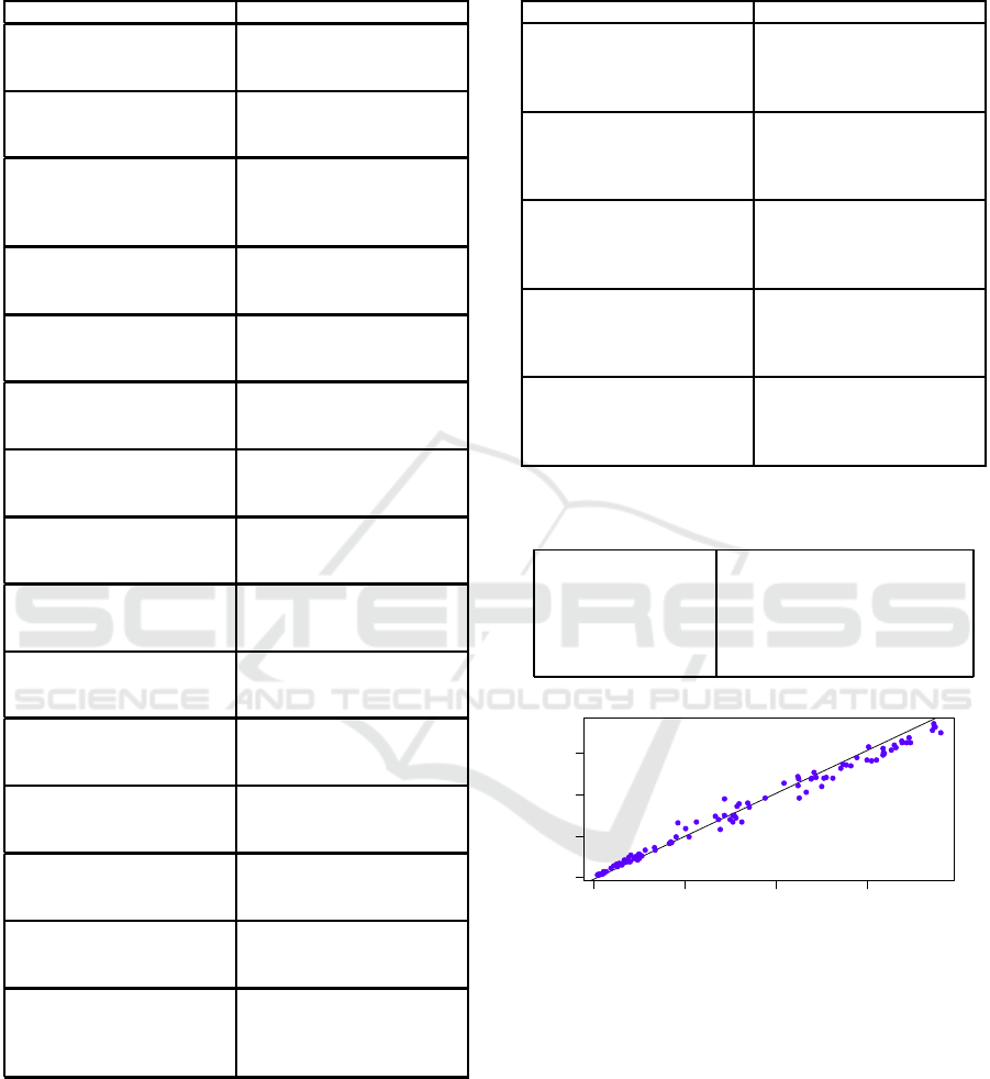
Table 6: Equations generated by applying M5P with CFS +
Random Search.
Condition Equation
AvgAirT <= 26.4 and WSpeed
<= 0.784
et0 = -0.0022 * MaxT + 0.002 *
AvgAirT + 0.0145 * WSpeed +
0.0024 * AvgSRad - 0.0115
WSpeed > 0.784 and AvgAirT
<= 24.718 and AvgSRad <=
6.249
et0 = -0.0057 * MaxT + 0.0054
* AvgAirT + 0.0097 * WSpeed +
0.001 * AvgSRad - 0.0088
AvgSRad > 6.249 et0 = -0.0103 * MinAtP - 0.0064
* MaxT + 0.0035 * AvgAirT +
0.0156 * WSpeed + 0.0052 *
AvgSRad + 6.1857
AvgAirT > 24.718 and AvgSRad
<= 6.963
et0 = -0.0069 * MaxT + 0.0065
* AvgAirT + 0.0138 * WSpeed +
0.0031 * AvgSRad - 0.0293
AvgSRad > 6.963 et0 = -0.0068 * MaxT + 0.0086
* AvgAirT + 0.0187 * WSpeed +
0.0023 * AvgSRad - 0.0787
AvgAirT > 26.4 and AvgSRad
<= 6.122 and AvgAirT <=
29.416
et0 = -0.0043 * MaxT + 0.0071
* AvgAirT + 0.0275 * WSpeed -
0.0024 * AvgSRad - 0.0932
AvgAirT > 29.416 and WSpeed
<= 0.822
et0 = -0.0021 * MaxT + 0.0044
* AvgAirT + 0.0617 * WSpeed +
0.0004 * AvgSRad - 0.1006
WSpeed <= 1.433 and AvgAirT
<= 32.715
et0 = -0.002 * MaxT + 0.009 *
AvgAirT + 0.0521 * WSpeed +
0.0004 * AvgSRad - 0.2454
AvgAirT > 32.715 et0 = -0.0023 * MaxT + 0.0083
* AvgAirT + 0.0602 * WSpeed +
0.0004 * AvgSRad - 0.2245
WSpeed > 1.433 and AvgAirT
<= 31.746
et0 = -0.0034 * MaxT + 0.0108
* AvgAirT + 0.0393 * WSpeed +
0.0004 * AvgSRad - 0.2582
AvgAirT > 31.746 et0 = -0.0041 * MaxT + 0.012 *
AvgAirT + 0.0551 * WSpeed -
0.0031 * AvgSRad - 0.294
AvgSRad > 6.122 and AvgAirT
<= 30.43 and WSpeed <= 1.851
et0 = -0.0062 * MaxT + 0.0074
* AvgAirT + 0.0407 * WSpeed +
0.002 * AvgSRad - 0.0994
WSpeed > 1.851 and MaxT <=
20.49
et0 = -0.0071 * MaxT + 0.0091
* AvgAirT + 0.0403 * WSpeed +
0.0016 * AvgSRad - 0.1248
MaxT > 20.49 et0 = -0.0067 * MaxT + 0.0089
* AvgAirT + 0.0357 * WSpeed +
0.0041 * AvgSRad - 0.1412
WSpeed <= 1.92 and WSpeed
<= 1.356
et0 = 0.003 * MinAtP - 0.0029
* MaxT + 0.0061 * AvgAirT +
0.0679 * WSpeed + 0.0008 *
AvgSRad - 1.9219
comparing the correlation of the models presented in
Table 5.
The approach proposed in this paper, the estima-
tion of ET
0
was performed for the collected climatic
variables of a weather station. We also applied a fea-
ture selection to reduce the dimensionality of the cli-
matic data. You can easily see in these experiments,
even with feature selection processing, the prediction
Table 7: Equations generated by applying M5P with CFS +
Random Search.
Condition Equation
WSpeed > 1.356 et0 = 0.0078 * MinAtP - 0.0041
* MaxT + 0.0068 * AvgAirT +
0.0643 * WSpeed + 0.0014 *
AvgSRad - 4.8287
AvgAirT <= 32.648 and WSpeed
<= 2.264
et0 = 0.0031 * MinAtP - 0.0066
* MaxT + 0.009 * AvgAirT +
0.0497 * WSpeed + 0.001 *
AvgSRad - 1.9765
WSpeed > 2.264 et0 = 0.0025 * MinAtP - 0.0065
* MaxT + 0.0103 * AvgAirT +
0.0499 * WSpeed + 0.0009 *
AvgSRad - 1.659
AvgAirT > 32.648 and WSpeed
<= 2.376
et0 = 0.0015 * MinAtP - 0.005
* MaxT + 0.0077 * AvgAirT +
0.0643 * WSpeed + 0.0015 *
AvgSRad - 1.0391
WSpeed > 2.376 et0 = 0.0018 * MinAtP - 0.0058
* MaxT + 0.0086 * AvgAirT +
0.0635 * WSpeed + 0.0018 *
AvgSRad - 1.2602
Table 8: Prediction Model generated by the Linear Regres-
sion with CFS + Random Search.
Linear Regres-
sion
et0 = -0.006 * MaxT
+ 0.0057 * AvgAirT
+ 0.0289 * WSpeed +
0.0055 * AvgSRad +
-0.0601
0.00 0.05 0.10 0.15
0.00 0.05 0.10 0.15
Weather Station
M5P: Feature Selection
R−squared: 0.989
Figure 3: Correlation between the estimated ET0 by M5P +
GeneticSearch and the weather station.
models achieved a high correlation degree between
the estimated ET
0
and its real value for the testing
dataset. So, it is worth reducing the data dimensional-
ity since the prediction models for ET
0
still have high
accuracy.
4 RELATED WORK
The use of predictive models to estimate the crop wa-
ter requirement has been studied by several authors
ICEIS 2017 - 19th International Conference on Enterprise Information Systems
276
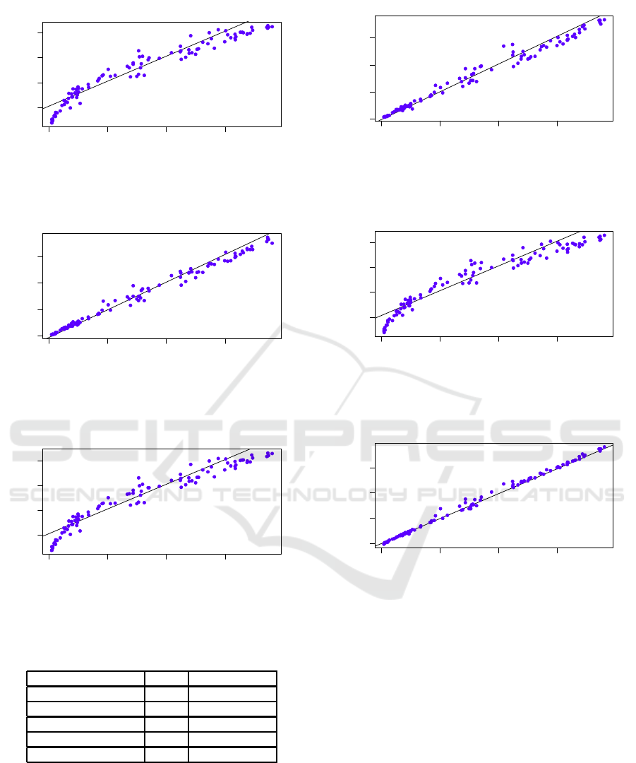
0.00 0.05 0.10 0.15
0.00 0.05 0.10 0.15
Weather Station
Linear Regression: Feature Selection
R−squared: 0.9302
Figure 4: Correlation between the estimated ET0 by Linear
Regression + GeneticSearch and the weather station.
0.00 0.05 0.10 0.15
0.00 0.05 0.10 0.15
Weather Station
M5P: Feature Selection
R−squared: 0.989
Figure 5: Correlation between the estimated ET0 by M5P +
ExhaustiveSearch and the weather station.
0.00 0.05 0.10 0.15
0.00 0.05 0.10 0.15
Weather Station
Linear Regression: Feature Selection
R−squared: 0.9308
Figure 6: Correlation between the estimated ET0 by Linear
Regression + ExhaustiveSearch and the weather station.
Table 9: Coefficient of determination (R
2
).
Algorithm M5P Linear Regression
CFS + Genetic Search 0.989 0.9302
CFS + Exhaustive Search 0.989 0.9308
CFS + BestFirst 0.9821 0.9262
CFS + RandomSearch 0.9957 0.9618
Without feature selection 0.9972 0.9666
and approached in different ways.
The paper (Hendrawan and Murase, 2011) pro-
poses irrigation system based on machine vision. The
system presents a predictive model which is used to
determine the amount of water required for the plants
with respect to its respective texture. In this way, the
stress caused by water was observed in a sunagoke
0.00 0.05 0.10 0.15
0.00 0.05 0.10 0.15
Weather Station
M5P: Feature Selection
R−squared: 0.9821
Figure 7: Correlation between the estimated ET0 by M5P +
BestFirst and the weather station.
0.00 0.05 0.10 0.15
0.00 0.05 0.10 0.15
Weather Station
Linear Regression: Feature Selection
R−squared: 0.9262
Figure 8: Correlation between the estimated ET0 by Linear
Regression + BestFirst and the weather station.
0.00 0.05 0.10 0.15
0.00 0.05 0.10 0.15
Weather Station
M5P: Feature Selection
R−squared: 0.9957
Figure 9: Correlation between the estimated ET0 by M5P +
RandomSearch and the weather station.
moss crop. Such observation was executed from pho-
tos and their respective color conversions. The au-
thors applied several algorithms of feature selection,
and the textures selected by each algorithm were used
as input to the classifier Back-Propagation Neural
Network. The study concluded the textures chosen by
the feature selection algorithms created accurate pre-
dictive models. Similar to (Hendrawan and Murase,
2011), our work proposes to use feature selection in
order to create a prediction model based on the set of
selected attributes. However, our proposal uses such
approach to estimate the reference evapotranspiration.
In (Xavier et al., 2016), the authors proposed a life
cycle model in data science to answer the question:
Can a simple approach be found to estimate poten-
Estimating Reference Evapotranspiration using Data Mining Prediction Models and Feature Selection
277
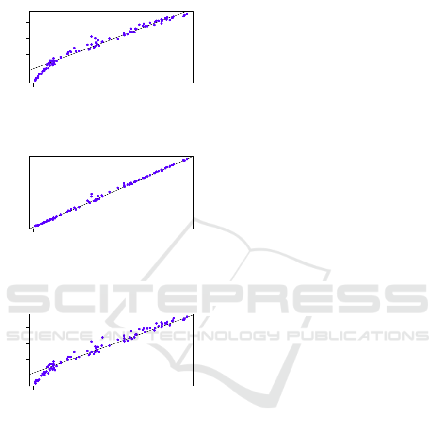
0.00 0.05 0.10 0.15
0.00 0.05 0.10 0.15
Weather Station
Linear Regression: Feature Selection
R−squared: 0.9618
Figure 10: Correlation between the estimated ET0 by Lin-
ear Regression + RandomSearch and the weather station.
0.00 0.05 0.10 0.15
0.00 0.05 0.10 0.15
Weather Station
M5P without Feature Selection
R−squared: 0.9972
Figure 11: Correlation between the estimated ET0 by M5P
without feature selection and the weather station.
0.00 0.05 0.10 0.15
0.00 0.10
Weather Station
Linear Regression without Feature Selection
R−squared: 0.9666
Figure 12: Correlation between the estimated ET0 by Lin-
ear Regression without feature selection and the weather
station.
tial evapotranspiration with an acceptable accuracy?
The experiments were performed by using historical
series (provided by INMET) of 263 meteorological
stations distributed in several cities of Brazil. The
authors used the M5P to create the models. To val-
idate the results, the authors compared the errors of
the models created by the M5P algorithm to the errors
generated using the Penman-Monteith model imple-
mented by R. They also examined the correlations of
the models. At the end of their study, they concluded
the models found out have a good accuracy and were
simpler than the Penman-Monteith method. Our pro-
posal also used the M5P to create predictive models.
However, we did not estimate the potential evapotran-
spiration. Moreover, we used different attribute selec-
tion algorithms for dimensionality reduction.
In (Sawalkar and Dixit, 2015), the authors ob-
tained meteorological data collected from the three
meteorological stations of United States of Geo-
logical Survey (USGS), Florida USA. For each
dataset, they calculate the evapotranspiration param-
eter (daily and monthly) using both the Penman-
Monteith method and the M5 decision trees. The
authors compared these models with their respective
correlation coefficients and associated errors. They
concluded the models generated by M5 algorithm es-
timated the evapotranspiration more accurately than
the Penman-Monteith method. Similarly, our pro-
posal used an algorithm based on M5 trees (M5P) to
create the prediction models. However, our proposal
differentiates by using feature selection algorithms for
dimensionality reduction.
In (Rahimikhoob, 2014), the authors created mod-
els to estimate the reference evapotranspiration by
using the M5 algorithm and also an artificial neural
network (ANN). They performed experiments using
data collected from four meteorological stations in-
stalled in the Sistan and Baluchestan provinces, Iran.
Based on the results, the authors concluded the ac-
curacy value of the model created by the M5 algo-
rithm was approximate to that of the model created by
ANN network. Moreover, they concluded the models
had a high degree of correlation with the data used.
Similar to (Rahimikhoob, 2014), our proposal created
prediction models using two different approaches to
estimate reference evapotranspiration. However, we
used Linear Regression as the second approach and
performed feature selection for data reduction.
5 CONCLUSIONS
In this paper, we aim at studying how to predict the
reference evapotranspiration value by using climatic
data. Moreover, these data are multidimensional and
might be not trivial to use a prediction model with
many attributes. Our solution applies feature selec-
tion methods in order to reduce the data dimensional-
ity and then investigate prediction models more accu-
rate. According to the results concerning the correla-
tions of the models, we can highlight that among the
four algorithms used (BestFirst, Random Search, Ex-
haustive Search, Genetic Search), the Random Search
selected the best set of attributes since it generates
the model with the highest correlation. Moreover,
M5P generated better models than traditional linear
regression. Since the Penman-Monteith method is
ICEIS 2017 - 19th International Conference on Enterprise Information Systems
278

too complex, the approach and the models reported
in this work could be very useful for farmers and
agronomists to estimate the evapotranspiration refer-
ence in locations with similar climatic conditions to
the city of Quixad´a. Moreover, other methods us-
ing data mining predictivemodels could be developed
based on the results introduced in this paper. As future
works, we aim to validate and improve our proposed
models for other datasets from other meteorological
stations.
REFERENCES
(2015). Irrigation Sector Reform. FAO. Corporative Web-
site.
(2015). Relat´orio de Conjuntura dos Recursos H´ıdricos no
Brasil 2014. Agˆencia Nacional de
´
Aguas.
(2016). PC200W 4.4.2. Campbell Scientific, Inc. Corpora-
tive Website.
Allen, R. G., Pereira, L. S., Raes, D., and Smith, M.
(1998). Crop evapotranspiration-guidelines for com-
puting crop water requirements-fao irrigation and
drainage paper 56. Fao, Rome, 300(9):D05109.
Fayyad, U., Piatetsky-Shapiro, G., and Smyth, P.
(1996). From data mining to knowledge discovery in
databases. AI magazine, 17(3):37.
Frizzone, J. A., de Souza, F., and Lima, S. C. R. V. (2013).
Manejo da irrigac¸˜ao: Quando, Quanto e Como Irri-
gar. INOVAGRI.
Garces-Restrepo, C., Vermillion, D., and Muoz, G. (2007).
Irrigation management transfer: Worldwide efforts
and results.
Hall, M., Frank, E., Holmes, G., Pfahringer, B., Reutemann,
P., and Witten, I. H. (2009). The weka data min-
ing software: an update. ACM SIGKDD explorations
newsletter, 11(1):10–18.
Hall, M. A. (1999). Correlation-based feature selection
for machine learning. PhD thesis, The University of
Waikato.
Hall, M. A. (2000). Correlation-based feature selection of
discrete and numeric class machine learning.
Hendrawan, Y. and Murase, H. (2011). Neural-intelligent
water drops algorithm to select relevant textural fea-
tures for developing precision irrigation system using
machine vision. Computers and Electronics in Agri-
culture, 77(2):214–228.
Karegowda, A. G., Manjunath, A., and Jayaram, M. (2010).
Comparative study of attribute selection using gain ra-
tio and correlation based feature selection. Interna-
tional Journal of Information Technology and Knowl-
edge Management, 2(2):271–277.
Liu, H. and Yu, L. (2005). Toward integrating feature
selection algorithms for classification and clustering.
IEEE Transactions on knowledge and data engineer-
ing, 17(4):491–502.
Rahimikhoob, A. (2014). Comparison between m5 model
tree and neural networks for estimating reference
evapotranspiration in an arid environment. Water re-
sources management, 28(3):657–669.
Sawalkar, N. and Dixit, P. (2015). Evapotranspiration mod-
eling using m5 model tree.
Wang, Y. and Witten, I. H. (1996). Induction of model trees
for predicting continuous classes. Working paper se-
ries.
Xavier, F., Tanaka, A. K., and Amorim, F. A. B. (2016).
Application of data science techniques in evapotran-
spiration estimation.
Estimating Reference Evapotranspiration using Data Mining Prediction Models and Feature Selection
279
