
Forecasting Public Transportation Capacity Utilisation Considering
External Factors
Fabian Ohler
1,2
, Karl-Heinz Krempels
1,2
and Sandra M
¨
obus
1
1
Informatik 5 (Information Systems), RWTH Aachen University, Aachen, Germany
2
CSCW Mobility, Fraunhofer FIT, Aachen, Germany
Keywords:
Passenger Demand Forecast, Public Transportation Forecast, Transit Passenger Volume Prediction.
Abstract:
Using a forecast of the public transportation capacity utilisation, the buses can be adapted to the demand to
avoid overfull buses leading to delays. An efficient utilisation of the buses at disposal can improve customer
satisfaction as well as economic efficiency. The basis for our forecasts provide fragmentary measurements of
passengers boarding and alighting buses at stops over the year 2015. In an attempt to improve the accuracy of
the forecast, several external factors (e. g. weather, holidays, cultural events) were incorporated. We tackle the
problem of forecasting public transportation capacity utilisation by forecasting the number of boarding and
alighting passengers. Then we use these to adjust previous passenger count and the result as input for next
forecast. Using multiple linear regression, support vector regression, and neural networks we evaluate different
ways to model the external factors. Best results were achieved by neural networks with a median absolute error
of ≈4.16 in the forecast passenger count. They were able to keep more than 80% of the forecasts within a
tolerance of 10 passengers. Since the error in the forecasts does not accumulate along the trips, chaining the
forecasts in the described way is a viable approach.
1 INTRODUCTION
In many domains, forecasts are important for plan-
ning and optimization. For public transportation com-
panies, forecasts of passenger load may be used to op-
timize their service planning. Their customers often
complain about crammed buses leading to crowding
and bad air during travels. Overfull buses also lead to
customers not being able to board the bus and having
to wait for follow-up buses. Additionally, the duration
of stays at bus stops is prolonged potentially leading
to delays. Thus, people switch to alternate modes of
travel like using a bike or car. For the bus service
providers, a loss of customers usually results in a fi-
nancial deficit. On the other hand, a lack of infor-
mation about the transportation demand may lead to
wasted capacities during times of low utilisation. In-
formation about passenger demand is a basis for bus
scheduling (Salzborn, 1972) and can help avoid the
aforementioned problems improving customer satis-
faction (Eboli and Mazzulla, 2007).
In times of interconnected vehicles, automatic ve-
hicle location systems, advanced traveller informa-
tion systems, etc., customers are used to being pre-
sented an expected time of arrival / departure for their
means of transportation. Enhancements regarding the
fidelity of this information might also be based on
a more accurate forecast of the passenger load espe-
cially during demand peaks.
In the project Mobility Broker
1
, multiple mobil-
ity services (e. g. bus, train, car-sharing, bike-sharing)
were integrated into one platform (Beutel et al.,
2016). For the sharing services, the limited availabil-
ity of its resources can prevent users from satisfying
their mobility needs, e. g. in case no bike is available
at the time the user wants to rent it. Therefore, the
user is informed about bike and vehicle availabilities
at the corresponding sharing stations via the mobile
app or the web browser. On the other hand, during de-
mand peaks also buses with high passenger capacity
reach their maximum load leading to unsatisfied mo-
bility needs. Including the passenger load into trav-
eller information systems can thus improve the travel-
ling experience by allowing the users of the system to
make informed choices regarding the mobility modes.
Therefore, in the context of the project Mobility Bro-
ker, we decided to investigate the possibility of fore-
casting the passenger load for buses.
1
https://mobility-broker.com/
300
Ohler, F., Krempels, K-H. and Möbus, S.
Forecasting Public Transportation Capacity Utilisation Considering External Factors.
DOI: 10.5220/0006345703000311
In Proceedings of the 3rd International Conference on Vehicle Technology and Intelligent Transport Systems (VEHITS 2017), pages 300-311
ISBN: 978-989-758-242-4
Copyright © 2017 by SCITEPRESS – Science and Technology Publications, Lda. All rights reserved

Due to the potential of predictions including the
aforementioned reasons, a lot of forecasting ap-
proaches have been developed ranging from simple
regression to time series models and data mining tech-
niques. In this paper, we compare different methods
to forecast the passenger load in buses. To do so, we
consider the number of passengers in a bus as the dif-
ference between the number of boarding and alighting
people in addition to the previous passenger count.
We develop a model to forecast the number of board-
ing and alighting people at a bus stop. The model
is trained using historical data exhibiting a relatively
low coverage compared to the amount of data that
could have been collected during the corresponding
time span. Additionally, we integrate multiple factors
that are likely to influence the passenger load into our
model.
After a short problem description in Section 2, we
survey the related work in Section 3. In Section 4,
we present our approach, which we thoroughly eval-
uate in Section 5. Section 6 gives a conclusion and
outlook.
2 PROBLEM DESCRIPTION
Forecasting means making a statement about future
events based on past observations. While definitive
statements about the future are rarely possible, math-
ematical models can be used to obtain an approxima-
tion. A forecasting model to determine the number
of passengers in a bus can be reduced to a model esti-
mating the number of people boarding a bus at a given
point in time. Using the same approach, one can fore-
cast the number of people alighting a bus at a given
point in time. Combining both information yields the
change in the passenger count at the considered stop
and tracking these changes starting from the first stop
accounts for the absolute passenger count.
The number of passengers in a bus at a specific
point in time is influenced by many different aspects,
some of them specific to the means of transport (e. g.,
position in route), others rather specific to the circum-
stances like bad weather (Singhal et al., 2014) or big
events (Friedman et al., 2001).
Commuters lead to a high transportation demand
on work days at specific times of the day. Similarly
pupils lead to demand peaks outside of holidays. Es-
pecially at the start of each semester, college students
tend to use public transportation a lot. Over the course
of the semester, the demand may vary.
Nice weather often encourages people to reach
their target by foot or bike instead of taking the bus.
The contrary is the case whilst rain or frost. Big
events may generally lead to a high demand and fluc-
tuation, but also to traffic jams, both of which has po-
tential to delay buses. Delays in turn also influence
the number of passengers in a bus, since some people
might miss connections or use other buses while oth-
ers reach the bus stop in addition to the usual demand.
Finally, the number of people in a bus can influence
the number of people able to board, e. g., since buses
have limited capacity, and to exit.
The relevant factors have to be modelled in a way
compatible with the employed algorithms yet retain-
ing enough information to be of value.
To train the models, we use historic data collected
via sensors above the bus doors counting the number
of passengers boarding and alighting the buses. Yet,
since not all vehicles serving the observed routes were
equipped with those sensors, our data set is a random
sample. The problem of choosing suitable algorithms
to work with the fragmented observation is also tack-
led in this paper.
3 RELATED WORK
Forecasting the number of passengers in a bus is an
example for demand forecasting. It is similar to fore-
casting energy demands in that both are time-variant,
periodic, and influenced by weather and holidays. In
the area of energy demand forecasting, many attempts
have been made since good forecasts can save huge
amounts of money in that domain and we thus lend a
relevant part of the literature from them.
We shortly present well-known forecasting ap-
proaches before weighing them up against each other
with respect to the problem instance. In (Alfares and
Nazeeruddin, 2002) suitable approaches are divided
into nine categories, augmented by additional two in
(Mansouri et al., 2014).
Multiple Regression. Multiple Regression models
statistical relations between the demand and exter-
nal factors via a linear combination. The regres-
sion coefficients can be determined using e. g., the
least squares method (Montgomery et al., 2015).
Yet, good results are usually only to be expected
in case of linear dependence.
Exponential Smoothing. Exponential Smoothing
relies on the assumption, that future observations
are more similar to observations of the recent past
than of those less recent. Based on historic data,
a function is modelled to predict future values
(Neusser, 2011).
Stochastic Time Series. Forecasting can also be
modelled using time series analysis. Here, the
Forecasting Public Transportation Capacity Utilisation Considering External Factors
301

prognosis is only based on past demand values
and external factors are not included into the
model. The most important model is the ARMA
model composed of the autoregressive (AR) and
the moving-average (MA) model. Using the MA
model to eliminate the white noise, the AR model
performs a regression based on the demand values
of the past. In case of non-stationary processes,
the ARIMA (autoregressive integrated moving-
average) model transforms it to a stationary pro-
cess by differentiation (Neusser, 2011).
Iteratively Reweighted Least-Squares The Iter-
atively Reweighted Least-Squares method is a
modification of the least-squares method, simi-
larly applicable to determine model parameters.
In (Mbamalu and El-Hawary, 1993), the authors
used this method to compute the coefficients of
an autoregressive model.
Adaptive Load Forecast. In Adaptive Load Fore-
cast models, the model parameters are automat-
ically adjusted to changing demand. An exam-
ple for a well-known model of this category is the
Kalman filter (Bastian, 1985).
ARMAX Model based on Genetic Algorithms.
The ARMAX model is an extension of the
ARMA model including external factors via
exogenous variables. In (Yang et al., 1995),
evolutionary programming is used to identify
the parameters of the model. Evolutionary
programming simulates the natural evolutionary
process to heuristically minimize the error of the
model.
Knowledge-based Expert Systems. Knowledge-
based Expert Systems are an artificial intelligence
approach to bestow upon a system the ability to
reason on its own. Based on facts and if-then-
rules processing the facts, these systems are able
to deduce new information. These systems can
use their rule set to forecast information inferred
from the encoded knowledge (Ertel, 2013).
Fuzzy Logic. Fuzzy Logic systems can model un-
known dynamic systems similar to expert systems
based on rules. Yet, instead of mapping values to
true or false, a membership function assigns val-
ues between 0 and 1. Similarities in the input data
are identified using first- and second-order differ-
ences (Adamy, 2007; Sachdeva and Verma, 2008).
Neural Networks. Neural Networks imitate the way
the human brain works. These networks consist of
nodes representing neurons and weighted edges.
Inputs are propagated through the network and the
output layer represents the result. Using (historic)
training data, the weights are adjusted to minimize
the deviation in the output – the network ‘learns’.
Afterwards, the network can be used for forecast-
ing. A downside of this approach is its black box
design – usually, the user is not able to recon-
struct how the network comes to its conclusions
(Adamy, 2007; Dai and Wang, 2007).
Support Vector Machines. Support Vector Ma-
chines are used for classification as well as for
regression. For classification purposes, the ma-
chine uses historic data to determine a hyperplane
that separates two classes as well as possible.
Regression is done by finding a region that is as
small as possible and concentrates all historic
data. Using a kernel function, even non-linear
regression is possible (Guo et al., 2006).
Hybrid Methods. Over the years, many of the afore-
mentioned approaches have been combined into
hybrid systems. Particularly successful were ap-
proaches combining neural networks and fuzzy
logic to so-called neuro-fuzzy systems (Jang,
1993). Furthermore, combinations of neural net-
works and support vector machines (Niu et al.,
2005) or fuzzy logic and expert systems have been
used for demand forecasting.
The methods presented are also used to forecast
demand for public transportation. For example, in
(Zhou et al., 2013) the ARIMA model and in (Xue
et al., 2015) the Kalman filter is used to forecast pas-
senger demand for buses. Both models are geared to-
wards time series and analyse stationarity, periodicity,
and volatility.
Yet, since the data available to us has the previ-
ously described characteristics of a random sample,
we don’t expect good results from using time series
analysis. The missing data would have to be interpo-
lated and the model would be trained with partially
defective data. We therefore don’t consider Expo-
nential Smoothing, Stochastic Time Series, ARMA,
ARIMA, and ARMAX models any further. As Itera-
tively Reweighted Least-Squares and Adaptive Load
Forecasting are just alternative methods to determine
the parameters for, e. g., Multiple Regression or the
ARMA model, these are neglected here, too.
Knowledge-based Expert Systems as well as
Fuzzy Logic have successfully been applied to energy
demand forecasting (Alfares and Nazeeruddin, 2002).
However, both systems heavily depend on knowledge
of domain experts which is not available to us at the
time of writing.
Using neural networks to forecast seems consid-
erably more promising, since the approach is toler-
ant with respect to vagueness, missing data and non-
linearity. In (Tsai et al., 2009), neural networks have
already been applied to forecast passenger load for
VEHITS 2017 - 3rd International Conference on Vehicle Technology and Intelligent Transport Systems
302

trains, yet only considering a very limited set of rather
coarse external factors. Furthermore, in (Mo and Su,
2009) a forecast for passenger demand for buses using
neural networks has been drafted incorporating time,
weekday and weather. In this paper, we include addi-
tional external factors into the model to evaluate the
enhancements with with respect to prognosis quality.
As mentioned before, Multiple Linear Regression
preforms best in case the results linearly depend on
the inputs. Even though this is not to be expected for
all factors considered, we will include this approach
to compare it to the more complex ones.
Non-linear dependencies can be modelled using
Support Vector Regression. In contrast to the neural
networks, this approach minimizes the upper bound
of the error instead of its mean. This can lead to better
results in many cases (Jang, 1993).
Even though hybrid systems are gaining more and
more attention in research (cf. (Alfares and Nazeerud-
din, 2002)), the application of these more complex
systems goes beyond the scope of this paper.
In the following, we will thus compare Neural
Networks, Support Vector Regression, and Multiple
Linear Regression.
4 APPROACH
Our forecast is based on models trained using historic
data compiled from several sources. Since the mea-
surement data we have at our disposal are for the city
of Aachen (Germany), the points considered as pos-
sible influences with respect to passenger demand are
specific to Aachen. The following aspects are consid-
ered as factors in the model:
• line and bus stop,
• number of passengers in the bus,
• delay,
• time,
• weekday,
• public holidays,
• school holidays,
• semester breaks of the RWTH Aachen University,
• weather,
• cultural events (CHIO
2
, Christmas market, fairs,
carnival, Weinsommer
3
, SeptemberSpecial
4
), and
2
http://www.chioaachen.de
3
http://www.weinsommer.de/aachen
4
http://www.aachenseptemberspecial.de
• home games of the local soccer club (Alemannia
Aachen).
The local transportation company ASEAG (Aach-
ener Straßenbahn und Energieversorgungs-AG) pro-
vided us with measurement data acquired in 2015 by
infrared sensors mounted above the doors of some
of their buses to determine the number of people
in the bus. This data also contains information
about the bus line and current stop, the delay of the
bus as well as current time and date. Times and
dates for public/school holidays, semester breaks and
the aforementioned cultural events and soccer games
were added manually. Using data from the German
Weather Service (DWD)
5
, we augmented the input
data with information about the weather. Accumu-
lating the data from the different sources and bring-
ing it into a homogeneous form finalised the data pre-
processing step.
In the data transformation and modelling steps,
the following points were taken into consideration:
Bus line and stop are used to partition the data. The
rest of the data has to be represented as real num-
bers. The number of people in the bus and the delay
are already given as natural numbers and the time is
modelled as the number of minutes since midnight.
For the weekday, we consider two different represen-
tations: It can either be modelled as a dummy vari-
able that is 1 if the data corresponds to a weekday and
0 if it belongs to a weekend. As an alternative, ev-
ery weekday can be considered on its own via seven
dummy variables for the seven different weekdays
(Monday to Sunday) and it is always the case, that
exactly one of them is 1. Similarly, the public holi-
days can be modelled using a dummy variable. Yet,
since we expect that demand in front of and after pub-
lic holidays differs from the usual demand, we also
consider modelling them using two variables holding
the number of days since the last and until the next
public holiday. School holidays, semester breaks, and
cultural events last for several days or even weeks.
As we expect increased demand at the start and end
of these periods (and their complements), in addi-
tion to the aforementioned dummy variable approach,
we consider the following alternative modelling: Us-
ing school holidays as an example, we create four
variables representing the amount of days since the
start of the holidays, days left of the current holidays,
days until the next holidays, and days since the end
of the last holidays. During holidays, the first two
of them are non-negative and the others are zero and
vice versa. The weather is modelled via temperature
in degree Celsius, relative humidity and precipitation
5
http://www.dwd.de/DE/leistungen/klimadatendeutsch
land/klarchivtagmonat.html
Forecasting Public Transportation Capacity Utilisation Considering External Factors
303

measured directly as real numbers. Additionally, a
variable holding the amount of minutes until kick-off
for soccer home games is introduced with values be-
coming negative after kick-off and being zero on days
without home games.
Hereby, we introduced several factors with two
different modelling strategies each (weekday, public
holidays, school holidays, semester breaks, cultural
events) resulting in different ways to model our input
data.
5 EVALUATION
We evaluated our approach using the statistics soft-
ware R (R Core Team, 2016). Various packages pro-
viding implementations for lots of statistical models
are available for R. Part of this collection is the mul-
tiple linear regression, which is implemented as lm
(linear models) in the stats package.
For the support vector regression, multiple imple-
mentations exist (Hornik et al., 2006). Because of its
additional function tune, the package e1071 (Meyer
et al., 2015) was chosen providing the function svm,
which also internally handles data scaling. Of the
four available kernels, the linear and radial kernels
were chosen for evaluation. Using predict, the trained
model can be used to forecast.
For neural networks, again, multiple implementa-
tions exist, out of which neuralnet (Fritsch and Guen-
ther, 2016) was chosen, since it is tailored to regres-
sion and can handle more than one hidden layer.
The aforementioned local public transport opera-
tor provided us with measurements for two bus lines:
For bus line 3A, there are 60682 measurement read-
ings, corresponding to about 2100 readings per stop.
33131 measurement readings were available for bus
line 3B, yielding about 1100 readings per stop. As al-
ready stated, not all vehicles were equipped with the
measurement devices.
After preprocessing the data and consolidating it
in a data warehouse it turned out that for public holi-
days, disproportionally few measurements were avail-
able even when considering that the bus frequency is
usually lower on holidays. Therefore, public holidays
were not considered as a separate factor.
This leaves us with sixteen ways to model our
factors. We numbered them consecutively from 1 to
16 such that they encode, how the factors are repre-
sented:
n = 1 +2
3
w + 2
2
h + 2
1
b + 2
0
c
Here, w, h, b, and c correspond to weekday, school
holidays, semester breaks, and cultural events, respec-
tively. In case a factor is modelled in the more elabo-
rate way, its variable is set to 1, otherwise (when it is
modelled via a dummy variable) it is 0. Hence, rep-
resentation 1 is the most simple and representation 16
the most complex one.
We evaluated five models using the approaches se-
lected with the first method being the multiple lin-
ear regression (MLR). Furthermore, we use the ε-
SVR as described in (Sch
¨
olkopf et al., 2000) with
the default value ε = 0.1 and the linear (SVR-L) as
well as the radial kernel (SVR-R). Since the parame-
ter C (and additionally γ for the radial kernel) signif-
icantly influence the results, we evaluate the models
for different parameter values. We choose C ∈ N
≤10
,
γ ∈ {0.2, 0.4, 0.6, 0.8, 1} and plot the value for the best
parameter (pair). In addition, we consider two neural
networks. A rather simple one (nnet1) with one hid-
den layer containing two neurons and a second one
(nnet2) with two hidden layers containing five neu-
rons in the first and three in the second layer. RPROP
was used to train the networks with a tolerance thresh-
old of 0.01 and at most 10 million iterations.
5.1 Forecasting Boarding and Alighting
Passenger Count per Stop
To compare the models and the different representa-
tions, for all stops of the bus lines 3A and 3B we
used a 10-fold cross-validation (cf. (Arlot and Celisse,
2010)) to determine the mean absolute error (MAE)
as well as the maximum and median of the absolute
error. The first and last stop were left out, since we
assume empty buses at the start and end of trips.
To allow for more general conclusions, the mean
of the MAE over all stops was determined for ev-
ery factor representation. Additionally, we trained the
models for the simplest factor representation using a
reduced set of data (5%, 10%, 25%, and 50% of the
measurement data). To evaluate the influence of the
amount of data available, we determined the MAE
for all stops of the bus line 3A using a 10-fold cross-
validation based on the reduced data sets.
For the various stops of a line, different pairs of
models and factor representations produce the lowest
MAEs. This is illustrated in Fig. 1 showing the MAE
of the forecast of alighting passengers at two exam-
ple stops of bus line 3B. For stop 2102, the best re-
sult is produced by the SVR using a linear kernel and
representation 7 while at stop 2133, the simple neural
network in combination with representation 9 leads to
the best results.
When considering the average MAE over all
stops, Fig. 2 illustrates that there are no major dif-
ferences between the various ways to represent the
VEHITS 2017 - 3rd International Conference on Vehicle Technology and Intelligent Transport Systems
304
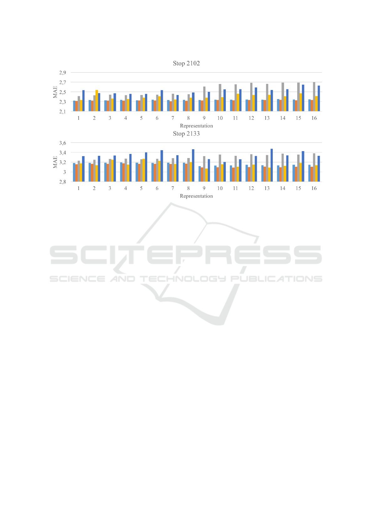
Figure 1: Mean absolute error in the forecast of the number of alighting passengers at three example stops of bus line 3B for
all 16 factor representations.
external factors. Only for the larger neural network
(nnet2), some of the errors are so large that they would
degrade the readability of the chart when fully plot-
ted. That’s why the average error values for represen-
tation 9 of the boarding passenger count for line 3A
(≈12.49) and for representation 13 of the boarding
passenger count for line 3B (≈7.96) are only hinted
at. In every case, choosing a more complex represen-
tation improves the MAE at most by a value of 0.03
when compared to the simplest representation.
For the more detailed comparison of the models,
we restrict ourselves to factor representation 1 tak-
ing into account the marginal differences between the
possible representations. Figure 3 illustrates the MAE
in the forecast of the alighting passenger count for
four exemplary stops of line 3B. As one can see, dif-
ferent models produce the smallest errors at the stops.
For the stops 2100 and 3171, the neural networks
seem favourable, but the support vector regression
performs better for the stops 3178 and 3508. How-
ever, the differences between the models in the MAE
values are rather small again.
Thus, we consider the overall values for all stops
once more. Table 1 shows the average values over all
stops of the mean, median, and maximum errors over
all trips for the simplest representation. For both bus
lines, the best mean and median error values are pro-
duced by the support vector regression using a radial
kernel. Here, most of the stops favoured the param-
eters C = 1 and γ = 0.2. Multiple linear regression
and the large neural network (nnet2) lead to the worst
results with respect to mean and median. When con-
sidering the average of the maximum error, the small
neural network (nnet1) performs best in three out of
four situations.
To evaluate the influence of the number of mea-
surement readings available, we randomly reduced
the available readings for bus line 3A to 5, 10, 25, and
50 percent of our data. Figure 4 shows the average
absolute errors in the forecast for the different mod-
els and data fractions. In most cases, smaller training
sets lead to worse results. This is especially true for
the neural networks, which degrade heavily for small
data sets. The least influence can be seen for the sup-
port vector regression.
5.2 Forecasting the Number of
Passengers in a Bus
In the following, we combine the information about
boarding and alighting passengers to determine the
number of passengers in a bus over a trip. To eval-
uate this approach, we examine 20 trips of bus line
3A and 19 trips of bus line 3B. The training set used
for a forecast consists of all historic information for
the corresponding stop and bus line minus the one
to be determined. For the origin stop of a trip, the
number of passengers in the bus when arriving at the
stop (possibly from previous trips of the vehicle; the
bus is empty most of the time) is taken from the mea-
surement readings. The forecast number of boarding
passengers is added, the forecast number of alighting
passengers is subtracted and the resulting value serves
as the number of passengers in the bus when arriv-
Forecasting Public Transportation Capacity Utilisation Considering External Factors
305
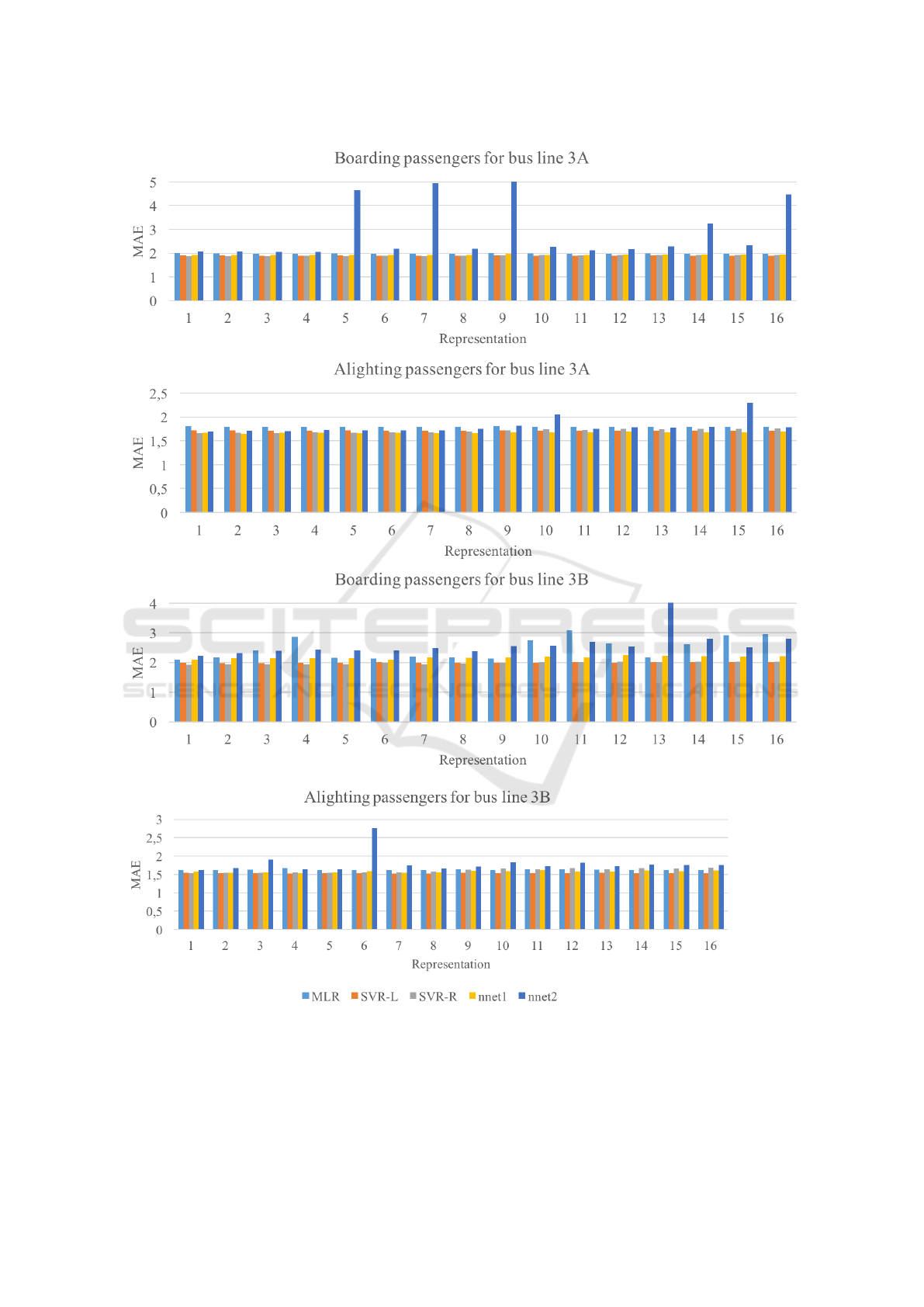
Figure 2: Average over the MAE of all stops with respect to the forecast of boarding and alighting passengers for the bus
lines 3A and 3B for all factor representations.
ing at the follow-up stop. For the remaining stops of
the trip, the forecast value resulting from the previ-
ous stop is used. In case the stop is a final stop where
no passenger ever entered according to historic data
or is an origin stop where no passenger ever left the
bus, this is incorporated in the forecast. Taking the
VEHITS 2017 - 3rd International Conference on Vehicle Technology and Intelligent Transport Systems
306

Table 1: Averages of the absolute errors in the forecast of boarding and alighting passengers for the bus lines 3A and 3B over
all stops for representation 1.
boarding passengers alighting passengers
mean median max mean median max
line 3A
MLR 2.01 1.55 24.48 1.81 1.35 22.31
SVR-L 1.91 1.32 25.50 1.73 1.20 23.92
SVR-R 1.86 1.30 25.37 1.66 1.16 25.73
nnet1 1.92 1.46 24.16 1.67 1.22 21.55
nnet2 2.07 1.44 153.68 1.69 1.20 44.91
line 3B
MLR 2.10 1.61 22.13 1.62 1.23 16.18
SVR-L 1.99 1.39 22.95 1.54 1.07 17.18
SVR-R 1.93 1.35 22.58 1.54 1.07 19.00
nnet1 2.09 1.53 21.96 1.57 1.11 16.47
nnet2 2.24 1.51 63.93 1.62 1.11 25.43
results from the previous section into account, the pa-
rameters for the support vector regression were set to
C = 1 and γ = 0.2, all other parameters and models
are unchanged.
Figure 3: Mean absolute error in the forecast of the number
of alighting passengers at four example stops of bus line 3B
for the simplest factor representation.
To compare the models, two trips of bus line 3A
were forecast and plotted together with the exact val-
ues in Figure 5. The external factors were represented
in the simplest way. For trip 41899, all models tend
to slightly underestimate the number of passengers
in the bus while for trip 54627, the opposite is the
case. Note that at the end of trip 41899, the bus is
not empty and the forecast is therefore not overridden
to zero in either case. Overall, the forecast does not
diverge from the exact values – so the error doesn’t
grow over time. Thus, our approach seems viable also
over longer time spans.
When factoring in the different representations,
the results for the two trips differed again (see Fig-
ure 6). The combination of representation and model
achieving best results depended on the trip. Com-
pared to the support vector regression using a ra-
dial kernel and the simplest representation which was
favoured in the previous stage, the MAE could be im-
proved by using another combination by about 4.44
and 3.66, respectively.
In Figure 7, all considered trips of both bus lines
are evaluated for all models and representations. The
median, 25%- and 75%-quartiles are plotted. For bus
line 3B, the best median absolute error was achieved
using SVR-R and representation 8 (an improvement
of about 14% compared to representation 1). When
looking at bus line 3A, the large neural network us-
ing representation 10 performed best gaining approx-
imately 27% accuracy over SVR-R in representation
1.
Since the capacity of a bus seems large compared
to the error values considered here, we also evaluated
the number of predictions that are within a tolerance
of up to n ∈ [1, 10] passengers. Representation 10 led
to the best results in nearly all situations including
n = 10. Therefore, Figure 8 only covers those values.
Table 2: Influence of integrating external factors on absolute
error in forecasting the number of people in the bus.
mean median
line 3A
nnet2 5.89 4.16
simple 7.60 5.82
minimal 10.49 8.00
line 3B
nnet2 6.74 5.05
simple 6.60 4.83
minimal 10.23 7.69
While the smaller neural network performed best
for bus line 3B for larger tolerance values, it was dom-
inated by SVR models for small tolerance values. For
bus line 3A, the larger neural network outperformed
all other models for all values of n.
We also evaluated an approach that for each stop
uses that pair of representation and model which min-
imizes the overall MAE for this stop. Yet, this ap-
proach yielded results similar to using a single model
and representation for all stops regarding the average
absolute error over the considered trips. Addition-
ally, we evaluated the influence of integrating exter-
Forecasting Public Transportation Capacity Utilisation Considering External Factors
307
Figure 4: Average over the MAE of all stops with respect to the forecast of boarding and alighting passengers for bus line 3A
in the simplest factor representation using reduced training data.
Figure 5: Exact and forecast number of passengers over the time of two example trips of line 3A (simplest representation).
Figure 6: MAE in the forecast of passengers in the bus over two example trips of line 3A for all representations.
nal factors. For this purpose, two further models were
trained only including time and weekday in its sim-
ple representation. The ‘simple’ model used radial
SVR with the aforementioned parameter values and
the ‘minimal’ model used MLR. Table 2 contains the
mean and median error values of the two models for
both bus lines and (for comparison) the values for the
larger neural network using representation 10. Here,
the error values for bus line 3B were slightly worse
for nnet2 than for the ‘simple’ approach. For line
3A (where about twice as many measurement read-
ings were available), the more sophisticated models
performed significantly better than the simpler ones.
6 CONCLUSION
In this paper, we evaluated multiple forecasting mod-
els to determine the number of passengers in a bus
over a trip. Several external factors (such as weather
and public holidays) were considered and different
ways to model them were presented. Using measure-
ment data for two bus lines, we evaluated the perfor-
mance of the models and the influence of the external
factors and the way they were represented. We started
by forecasting the number of boarding and alighting
passengers at a bus stop. Combined with the number
of passengers in the bus previous to the stop, these
numbers give us the passenger count in the bus after
the stop. Using this approach along trips does not lead
to accumulated errors and is thus feasible. In conclu-
sion, the neural network with two hidden layers using
VEHITS 2017 - 3rd International Conference on Vehicle Technology and Intelligent Transport Systems
308
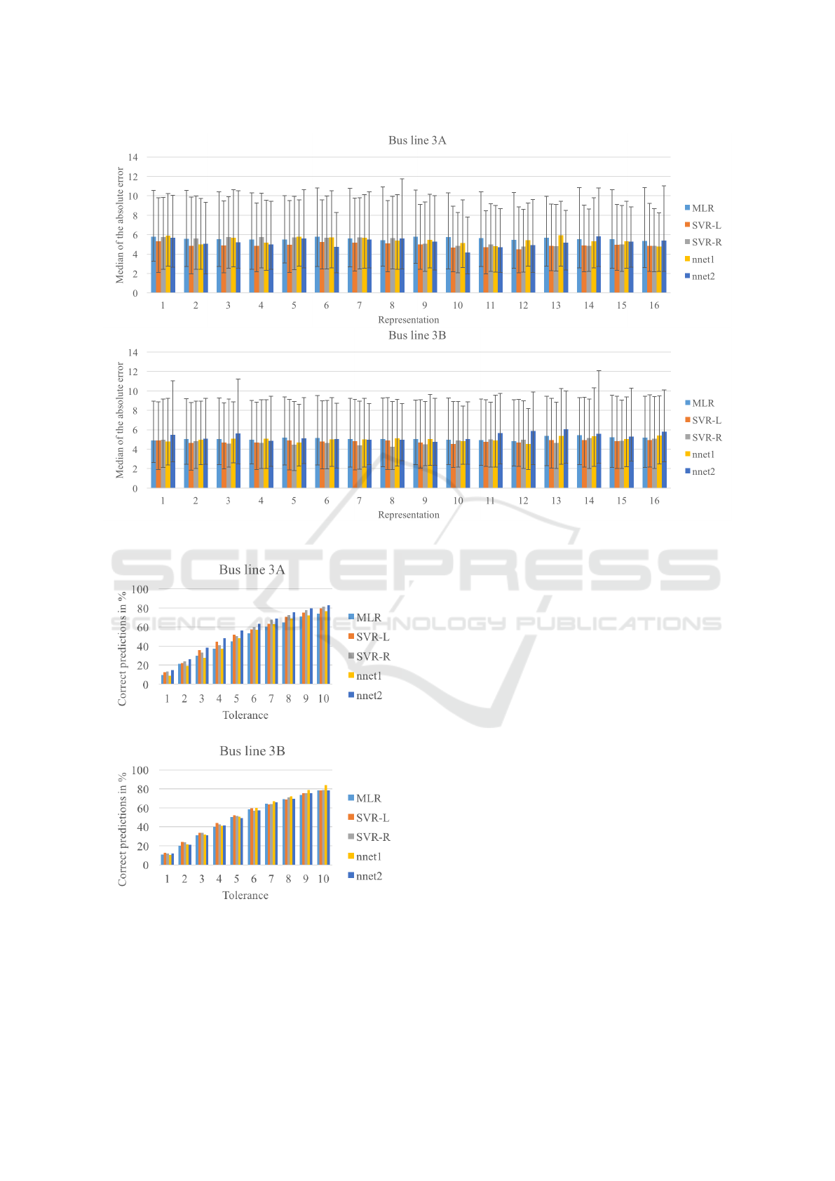
Figure 7: Quartiles (25%, 50%, 75%) of the absolute error values in the forecast of passengers in the bus for both bus lines.
Figure 8: Average percentage of forecasts correct within
increasing tolerance values for representation 10.
representation 10 seems to be a good fit for the avail-
able data set for bus line 3A. Representation 10 mod-
els school holidays and semester breaks via dummy
variables, but uses the more elaborate version for the
factors weekday and cultural events. With more data
available (also for bus line 3B), neural networks are
promising to perform even better (see Figure 4). Con-
sidering the external factors, the different representa-
tions have an impact on the accuracy of the predic-
tions, especially for the larger neural network. To
integrate the external factors into the models seems
to be beneficial especially when more data is avail-
able to overcome possible overfitting. When allowing
for a tolerance of 10 passengers for the forecast, the
neural networks again achieve good results and out-
perform the other models reaching adequate results in
over 80% of the cases (having passenger counts of up
to 139 in the data, a tolerance of 10 passengers seems
sufficiently small).
While we only considered two different neural
networks, other variations in the number of layers and
neurons are possible. Additionally, hybrid methods
often lead to amazingly precise forecasts. Thus, in-
vestigating well-fitting candidates constitute the next
step in our future research. Selecting suitable training
data could also be improved, possibly by employing
classifications methods. Furthermore, other represen-
tations for external factors could be studied, e. g., cat-
egorising the weather instead of taking raw inputs. On
the other hand, it might me worthwhile to differenti-
ate between the cultural events considered.
As we only had data for two bus lines going into
Forecasting Public Transportation Capacity Utilisation Considering External Factors
309

opposite directions, we treated them separately. Con-
sidering the whole bus network at once may enable
the model to learn about the interdependencies be-
tween different bus lines. Additionally, the scope can
be magnified by integrating trains or other modes of
transportation.
ACKNOWLEDGMENTS
This work was partially funded by German Federal
Ministry of Economic Affairs and Energy (BMWi)
for the project Mobility Broker (01ME12136) as well
as for the project Digitalisierte Mobilit
¨
at – Die Offene
Mobilit
¨
atsplattform (DiMo-OMP).
REFERENCES
Adamy, J. (2007). Fuzzy Logik, Neuronale Netze und Evo-
lution
¨
are Algorithmen. Shaker.
Alfares, H. K. and Nazeeruddin, M. (2002). Electric load
forecasting: Literature survey and classification of
methods. Int. J. Systems Science, 33(1):23–34.
Arlot, S. and Celisse, A. (2010). A survey of cross-
validation procedures for model selection. Statist.
Surv., 4:40–79.
Bastian, J. (1985). Optimale Zeitreihenprognose: empir.
Probleme u. L
¨
osungen. PhD thesis, University of
Giessen, Gießen, Germany.
Beutel, M. C., G
¨
okay, S., Kluth, W., Krempels, K.-H.,
Ohler, F., Samsel, C., Terwelp, C., and Wiederhold,
M. (2016). Information integration for advanced travel
information systems. Journal of Traffic and Trans-
portation Engineering, 4(4).
Dai, W. and Wang, P. (2007). Application of pattern recog-
nition and artificial neural network to load forecasting
in electric power system. In Third International Con-
ference on Natural Computation (ICNC 2007), vol-
ume 1, pages 381–385.
Eboli, L. and Mazzulla, G. (2007). Service quality attributes
affecting customer satisfaction for bus transit. Journal
of public transportation, 10(3):2.
Ertel, W. (2013). Grundkurs k
¨
unstliche Intelligenz: eine
praxisorientierte Einf
¨
uhrung. Springer-Verlag.
Friedman, M. S., Powell, K. E., Hutwagner, L., Graham,
L. M., and Teague, W. G. (2001). Impact of changes
in transportation and commuting behaviors during the
1996 summer olympic games in atlanta on air quality
and childhood asthma. JAMA, 285(7):897–905.
Fritsch, S. and Guenther, F. (2016). neuralnet: Training of
Neural Networks. R package version 1.33.
Guo, Y.-C., Niu, D.-X., and Chen, Y.-X. (2006). Support
vector machine model in electricity load forecasting.
In 2006 International Conference on Machine Learn-
ing and Cybernetics, pages 2892–2896. IEEE.
Hornik, K., Meyer, D., and Karatzoglou, A. (2006). Support
vector machines in r. Journal of statistical software,
15(9):1–28.
Jang, J. R. (1993). ANFIS: adaptive-network-based fuzzy
inference system. IEEE Trans. Systems, Man, and Cy-
bernetics, 23(3):665–685.
Mansouri, V. et al. (2014). Neural networks in electric
load forecasting: A comprehensive survey. Jour-
nal of Artificial Intelligence in Electrical Engineering,
3(10):37–50.
Mbamalu, G. and El-Hawary, M. (1993). Load forecasting
via suboptimal seasonal autoregressive models and it-
eratively reweighted least squares estimation. IEEE
Transactions on Power Systems, 8(1):343–348.
Meyer, D., Dimitriadou, E., Hornik, K., Weingessel, A., and
Leisch, F. (2015). e1071: Misc Functions of the De-
partment of Statistics, Probability Theory Group (For-
merly: E1071), TU Wien. R package version 1.6-7.
Mo, Y. and Su, Y. (2009). Neural networks based
real-time transit passenger volume prediction. In
Power Electronics and Intelligent Transportation Sys-
tem (PEITS), 2009 2nd International Conference on,
volume 2, pages 303–306. IEEE.
Montgomery, D. C., Peck, E. A., and Vining, G. G. (2015).
Introduction to linear regression analysis. John Wiley
& Sons.
Neusser, K. (2011). Die sch
¨
atzung vektor-autoregressiver
modelle. In Zeitreihenanalyse in den Wirtschaftswis-
senschaften, pages 191–195. Springer.
Niu, D.-X., Wanq, Q., and Li, J.-C. (2005). Short term
load forecasting model using support vector machine
based on artificial neural network. In 2005 Interna-
tional Conference on Machine Learning and Cyber-
netics, volume 7, pages 4260–4265. IEEE.
R Core Team (2016). R: A Language and Environment for
Statistical Computing. R Foundation for Statistical
Computing, Vienna, Austria.
Sachdeva, S. and Verma, C. M. (2008). Load forecasting
using fuzzy methods. In Power System Technology
and IEEE Power India Conference, 2008. POWER-
CON 2008. Joint International Conference on, pages
1–4. IEEE.
Salzborn, F. J. M. (1972). Optimum bus scheduling. Trans-
portation Science, 6(2):137–148.
Sch
¨
olkopf, B., Smola, A. J., Williamson, R. C., and Bartlett,
P. L. (2000). New support vector algorithms. Neural
Computation, 12(5):1207–1245.
Singhal, A., Kamga, C., and Yazici, A. (2014). Impact of
weather on urban transit ridership. Transportation Re-
search Part A: Policy and Practice, 69:379 – 391.
Tsai, T., Lee, C., and Wei, C. (2009). Neural network
based temporal feature models for short-term railway
passenger demand forecasting. Expert Syst. Appl.,
36(2):3728–3736.
Xue, R., Sun, D. J., and Chen, S. (2015). Short-term
bus passenger demand prediction based on time se-
ries model and interactive multiple model approach.
Discrete Dynamics in Nature and Society, 2015.
Yang, H.-T., Huang, C.-M., and Huang, C.-L. (1995). Iden-
tification of armax model for short term load forecast-
ing: an evolutionary programming approach. In Pro-
VEHITS 2017 - 3rd International Conference on Vehicle Technology and Intelligent Transport Systems
310

ceedings of Power Industry Computer Applications
Conference, pages 325–330.
Zhou, C., Dai, P., and Li, R. (2013). The passenger de-
mand prediction model on bus networks. In Ding, W.,
Washio, T., Xiong, H., Karypis, G., Thuraisingham,
B. M., Cook, D. J., and Wu, X., editors, 13th IEEE
International Conference on Data Mining Workshops,
ICDM Workshops, TX, USA, December 7-10, 2013,
pages 1069–1076. IEEE Computer Society.
Forecasting Public Transportation Capacity Utilisation Considering External Factors
311
