
Stochastic Simulation of Non-stationary Meteorological Time-series
Daily Precipitation Indicators, Maximum and Minimum Air Temperature
Simulation using Latent and Transformed Gaussian Processes
Nina Kargapolova
1,2
1
Institute of Computational Mathematics and Mathematical Geophysics, Pr. Lavrentieva 6, Novosibirsk, Russia
2
Novosibirsk State University, Novosibirsk, Russia
Keywords: Stochastic Simulation, Non-stationary Random Process, Air Temperature, Daily Precipitation, Extreme
Weather Event.
Abstract: In this paper a stochastic parametric simulation model that provides daily values for precipitation indicators,
maximum and minimum temperature at a single site on a yearlong time-interval is presented. The model is
constructed on the assumption that these weather elements are non-stationary random processes and their
one-dimensional distributions vary from day to day. A latent Gaussian process and its threshold
transformation are used for simulation of precipitation indicators. Parameters of the model (parameters of
one-dimensional distributions, auto- and cross-correlation functions) are chosen for each location on the
basis of real data from a weather station situated in this location. Several examples of model applications are
given. It is shown that simulated data may be used for estimation of probability of extreme weather events
occurrence (e.g. sharp temperature drops, extended periods of high temperature and precipitation absence).
1 INTRODUCTION
For solution of different applied problems in such
scientific areas as hydrology, agricultural
meteorology and population biology, it is quite often
necessary to take into account statistical properties
of different meteorological processes. For example,
it may be necessary to consider probability of
occurrence of meteorological elements combinations
contributing to forest fires spread, probability of
frost occurrence in spring and summer, average
number of dry days, etc. Since real data samples are
usually small, real data based statistical investigation
of rare and extreme weather events is in most cases
unreliable. Therefore, instead of small real data
samples it is necessary to use samples of simulated
data.
In this regard, in recent decades a lot of scientific
groups all over the world work at development of
so-called "stochastic weather generator". At its core,
"generators" are software packages that allow
numerically simulate long sequences of random
numbers having statistical properties, repeating the
basic properties of real meteorological series. Most
often series of surface air temperature, daily
minimum and maximum temperatures, precipitation
and solar radiation are simulated (Furrer, 2007;
Kargapolova, 2012; Richardson, 1981; Richardson,
1984; Semenov, 2002). Not only single-site time
series, but also spatial and spatio-temporal
meteorological random fields are simulated with the
use of "weather generators" (Kleiber, 2012;
Ogorodnikov, 2013; Kargapolova, 2016). It should
be noted that practically all “weather generators”
possess same drawback: a model that describes well
main properties of a weather process over some
region or at several locations may be totally
unsuitable over another region (with different
physiographic characteristics). At the same time,
models that reproduce well characteristics of a
weather process on a relatively short time-interval (a
week, a month) may not be applicable for longer
periods of time (season, year) and vice versa. It
means that for each specific applied problem
solution it is always a good idea to try several
“weather generators” and then to choose the one that
“works” better.
In this paper a stochastic parametric simulation
model that provides daily values for precipitation
indicators, maximum and minimum temperature at a
single site on a yearlong time-interval is presented.
The model is constructed on the assumption that
Kargapolova, N.
Stochastic Simulation of Non-stationary Meteorological Time-series - Daily Precipitation Indicators, Maximum and Minimum Air Temperature Simulation using Latent and Transformed
Gaussian Processes.
DOI: 10.5220/0006358801730179
In Proceedings of the 7th International Conference on Simulation and Modeling Methodologies, Technologies and Applications (SIMULTECH 2017), pages 173-179
ISBN: 978-989-758-265-3
Copyright © 2017 by SCITEPRESS – Science and Technology Publications, Lda. All rights reserved
173
these weather elements are non-stationary random
processes and their one-dimensional distributions
vary from day to day. A latent Gaussian process and
its non-linear transformation (so called threshold
transformation) are used for simulation of
precipitation indicators. Parameters of the model are
chosen for each location on the basis of real data
from a weather station situated in this location.
Several examples of model applications are given. It
is shown that simulated data may be used for
estimation of probability of extreme weather events
occurrence.
2 MODEL DESPRIPTION
In this section a formal theoretical description of a
considered stochastic model is given. Assumptions
about properties of a real weather proses that were
used for model construction are specified.
A model is constructed for simulation of joint
time-series on twelve-month time interval. It is
supposed that one-dimensional distribution of daily
maximum and minimum temperature are Gaussian.
This assumption is in good agreement (in sense of
2
-criteria) with long-term observation data from
weather stations. Parameters of these Gaussian
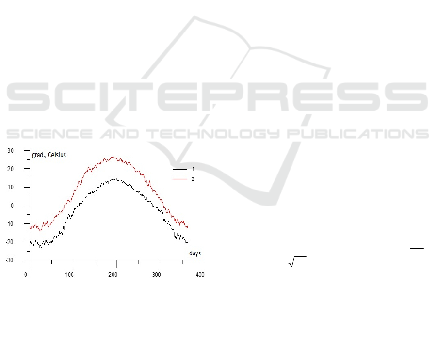
distribution vary from day to day. Figure 1 illustrates
variation of daily maximum and minimum
temperature sample average on a yearlong interval.
Figure 1: Sample average of daily minimum (1) and
maximum (2) temperature. Years of observation: 1976 –
2009. Novosibirsk, Russia.
Daily precipitation indicator in a day number
j, j 1, N is defined as 1 if amount of precipitation
during this day in more of equal than
0.1 mm and as
0 otherwise. It is supposed that
N
365 (for
convenience data for February 29 is not taken into
consideration). This means that daily precipitation
indicator is a binary random process. Joint time-
series of mentioned above weather elements are
assumed to be non-stationary on twelve-month time
interval.
Each simulated model trajectory is a matrix
TTT
MI,A,E
, where column-vector
T
T
12 N
II,I,,I
is a vector whose component
j
I
is daily minimum air temperature in a day
number
j ,
T
T
12 N
AA,A,,A
is a vector of
daily maximum temperatures and column-vector
T
T
12 N
EE,E,,E
is a vector of daily
precipitation indicators.
Elements of a joint time-series
M are calculated
with the help of transformations
II I
j
jj j
AA A
j
jj j
E
j
j
j
E
j
j
I,
A,
1, c ,
E
0, c ,
(2.1)
where vectors
IAIA
11 11
IAIA
22 22
IAIA
NNNN
,,,
are mean and standard deviation vectors, j1,N .
Threshold values
j
c
are defined from equations
j
c
2
jj
1t
PE 1 exp dt p,j 1,N.
2
2
Values of
IAIA
j
jj jj
,,,,p
are estimated on a
basis of real data from a weather station. It is
obvious that such way of model parameters
definition make it possible to take into account
seasonal variations of real weather processes It
should be noted that for all
j1,N equality
j
c0
is true if and only if
j
p
0.5
, inequalities
j
c0
and
j
p
0.5 are equivalent. Hereafter it is supposed
SIMULTECH 2017 - 7th International Conference on Simulation and Modeling Methodologies, Technologies and Applications
174

that
ii
p
0, p 1, i 1, N. Variables
IAE
jj j
,,
are components of a joint Gaussian process
TTT
IAE
,,
with zero mean and
specific correlation matrix
II IA IE
AI AA AE
EI EA EE
GG G
GG G G .
GG G
Matrix G must be such that a process
TTT
I,A,E
after transformation (2.1) has a
correlation matrix
II IA IE
AI AA AE
EI EA EE
RR R
RR R R ,
RR R
that is equal to sample correlation matrix. Method of
matrix G calculation is described below. Dimension
of matrixes
G and
R
is 1095 1095 (3N 3N
).
Element
XY
ri,j of a matrix block
XY
R is a
correlation coefficient between
i
X and
j
Y
(
X,Y I,A,E , i,j 1,2, ,N ). Element
XY
gi,j is corresponding to
XY
ri,j correlation
coefficient of a Gaussian process.
Let’s take a closer look at the matrix
G and find
equations that define this matrix when the matrix
R
is given. In (Ogorodnikov, 2009) a special case of
such equations was considered. Normalisation of
two correlated Gaussian random variables doesn’t
change a correlation coefficient between them,
which implies
II II AA AA
IA IA AI AI
GR,G R,
GR,GR.
(2.2)
Definition of a correlation coefficient leads to
equations
ij i j
IE
ij
EI E EI EE
ri,j
DI DE
(2.3)
IE
2
j
jj
gi,j
exp c 2 , i, j 1, N.
2p 1 p
These equations fully define matrix
IE
G . Matrixes
EI AE EA
G,G ,G are defined in a similar way. Since
ij ij
EE
iijj
EE
ij i j
ij
PE 1,E 1 pp
ri,j ,
p1p p1p
P E 1, E 1 P c , c , i, j 1, N
following equalities hold for i, j 1, N & i j,
ijEE ij
EE
iijj
F c ,c ,g i,j p p
ri,j ,
p1p p1p
(2.4)
where
2
hk
22
2
1
Fh,k,
21
1
exp x 2 xy y dxdy.
21
Obviosly,
EE EE
ri,igi,i1,i1,N.
It should be noted that equations (2.4) don’t have
any analytical solutions, but it is possible to solve
them numerically. So, equations (2.2) – (2.4) define
matrix
G and, finally, we may formulate the
simulation algorithm.
Algorithm:
Step 1. Estimate
IAIA
j
jj jj
,,,,p,j1,N
on
a basis of real data.
Step 2. Solving equations (2.2) – (2.4) define
matrix
G .
Step 3. Simulate required number of trajectories
of a joint Gaussian process
with zero mean and
correlation matrix
G .
Step 4. Using equalities (2.1) transform
trajectories of a Gaussian processes into trajectories
of a non-Gaussian process
TTT
M I ,A ,E
.
If verification of obtained trajectories gives
satisfying result, these trajectories may be used for
study of rare / extreme events.
Remark 1. Due to a physical sense of daily
minimum and maximum temperatures, an inequality
jj
IA
must be true for all
j1,N
. But
transformation (2.1) doesn’t guarantee it. This
means that one must eliminate from consideration all
trajectories in which this inequality violates. In
Stochastic Simulation of Non-stationary Meteorological Time-series - Daily Precipitation Indicators, Maximum and Minimum Air
Temperature Simulation using Latent and Transformed Gaussian Processes
175

practice, it is typical that
IA
jj
and
IA
jj
,
are
relatively small, so usually there are few trajectories
with
jj
IA
.
Remark 2. Equations (2.4) are solved
numerically, so some computational errors may
appear. These errors influence on the matrix
G and
it may happen that obtained matrix
G is not
positively-defined. In this case before a Gaussian
process simulation a normalisation of the matrix
G
must be done (see, Ogorodnikov, 1996). There are a
lot of algorithms for simulation of a Gaussian
process with given correlation matrix. The most
common are algorithms based on
LU decomposition of the correlation matrix and
on its spectral representation.
Remark 3. Numerical solution of equations (2.4)
is a time-consuming problem. There is a way to
reduce computational time. So-called Owen’s
formulas (Owen, 1956) give a representation of
function
Fh,k,
via one-dimensional integrals:
ijEE i j
i1 j2
11
F c ,c ,g i,j c c
22
1
Tc,a Tc,a ,
2
if
ij
c0,c0 or
ij
c0,c0, and
ijEE i j
i1 j2
11
F c ,c ,g i,j c c
22
Tc,a Tc,a ,
if
ij
c0,c0
or
ij
c0,c0,
where
i
c
2
i
0
1
c exp t 2 dt,
2
22
a
2
0
j i EE i j EE
12
22
ij
EE EE
c1t
1dt
Tc,a exp ,
22
1t
c cg i,j c cg i,j
a,a .
c1gi,j c1gi,j
This representation together with the fact that
ii
1
p
c,i1,N
2
let to replace equations (2.4) with equations
ijij
EE
iijj
i1 j2
iijj
11
pppp
22
ri,j
p1p p1p
Tc,a Tc,a
,
p1p p1p
(2.5a)
if
ij
cc 0
,
ij ij
EE
iijj
i1 j2
iijj
111
p
ppp
222
ri,j
p
1p p1p
T c ,a T c ,a
p1p p1p
(2.5b)
if
ij
cc 0
,
EE
j
2
EE
EE
jj
gi,j
2T c ,
1g i,j
ri,j ,
p1p
(2.5c)
if
ij
c0,c0,
EE
i
2
EE
EE
ii
gi,j
2T c ,
1g i,j
ri,j
p1p
(2.5d)
if
ij
c0,c0
and
EE
EE
2arcsing i,j
ri,j
(2.5e)
if
ij
cc0
.
Numerical experiments show that computational
time required for solution of equations (2.5a) –
(2.5e) is approximately 4 times less than
computational time required for solution of
equations (2.4). This is due to the fact that
computation of a one-dimensional integral is much
simpler than computational of a bivariate integral.
Remark 5. In some numerical experiments,
obtained matrix G was ill-conditioned and didn’t let
accurate simulation of a Gaussian process. It calls
for further investigations to find out conditions when
SIMULTECH 2017 - 7th International Conference on Simulation and Modeling Methodologies, Technologies and Applications
176

matrix
G is ill-conditioned. Ways of matrix
correction are also have to be found.
Remark 6. Since correlation coefficients
EE
gi,j
may be found from equations (2.4) (or
(2.5a) – (2.5e)) independently from each other and
trajectories of the Gaussian process are also
simulated independently, parallel computing
technologies may be easily applied for simulation of
the process
TTT
MI,A,E
.
3 NUMERICAL EXPERIMENTS
Described above stochastic model was used for
simulation of joint meteorological non-stationary
time-series on more than 50 weather stations situated
in different climatic zones in Russia. Verification of
the model shows that the model gives satisfactory
results for most of the stations. Here is an example
of a process characteristic that was used for the
model verification. Average numbers of days in a
month, when minimum temperature is below
0
o
C
and maximum temperature is above
0
o
C
(
jj
I0,A0), estimated on basis of real and
simulated data, were compared. This characteristic is
not the model input parameter, so it can be used for
verification. Table 1 presents values of this
characteristic. It can be seen from Table 1, that the
model reproduces this characteristic accurately (up
to a statistical mistake).
Table 1: Average number of days with
jj
I0,A0
. St.
Petersburg, Russia.
Month
Average number of days
Real data Simulated data
Octobe
r
4.7 4.9
Novembe
r
8.9 9.1
Decembe
r
5.7 5.3
January 9.3 9.4
February 7.7 7.4
March 16.3 16.8
Since the model is adequate to real weather
processes, it may be used for study of rare / extreme
events. Here are several examples. Hereafter all
estimations on basis of real data were done for years
of observation from 1976 to 2009 and estimations
based on simulated data were done over
6
10
trajectories.
First considered characteristic is a probability of
low temperatures and light frosts in spring and
summer. These weather events may negatively
influence on open-ground planted crop species.
Since different species have different resistance to
frost, it is necessary to take probability of low
temperatures and light frosts into account when
choosing a varieties or species of plants. Formally,
considered characteristic may be written as
j
PI
when j varies from 121 (May 1) to 243
(August 31). Here
o
C (deg. Celsius) is a given
temperature level. Table 2 presents estimations of
j
PI
obtained on basis of real and simulated
data. For real and simulated data estimations two
and three, respectively, fraction digits are
significant. During years of observation, there were
no days in considered period with temperature below
6
o
C (this is subminimum temperature for most of
plants species), but it doesn’t mean that such
temperature drop is impossible. Simulated data
provides an estimation of probability of this rare and
severe weather condition.
Table 2: Estimations of
j
PI
obtained on basis of
real and simulated data. Novosibirsk, Russia.
o
C
j
P I , j 121,234
Real data Simulated data
2 0.081 0.085
0 0.030 0.031
-2 0.014 0.013
-6 0.000 0.001
Table 3: Average number of summer time-intervals lasting
k days, with absence of precipitation and daily minimum
temperature above 20
o
C. Astrakhan, Russia.
Period
length, days
Average number of time-intervals
Real data Simulated data
k=1 5.3 5.72
k=2 2.0 2.20
k=4 0.7 0.76
k=5 0.6 0.59
k=6 0.0 0.53
k=8 0.0 0.37
k=9 0.3 0.32
k=10 0.1 0.09
Another weather event that may be dangerous
both to individuals and to agricultural industry is
long-term combination of high air temperature and
absence of precipitation. Such combination may
negatively influence on individuals’ health and may
cause soil drying up. Table 3 presents average
number of time-intervals lasting
k days, when daily
minimum temperature was above 20
o
C and there
were no precipitations (only significant digits are
Stochastic Simulation of Non-stationary Meteorological Time-series - Daily Precipitation Indicators, Maximum and Minimum Air
Temperature Simulation using Latent and Transformed Gaussian Processes
177

given). Averaging was done over summer months.
Once again, described in the paper model reproduces
this characteristic for short time-intervals
satisfactory, so model results for longer time-
intervals may be considered as reasonable.
Finally, let’s consider such unpleasant weather
event as sharp temperature drop or rise during one
day (formally,
jj
AI, where
o
C is given
level.). Numerical analysis shows that this
characteristic is reproduced well for
5,14 . For
14
o
C real data estimations are unreliable. This
means that for applied problems solutions it is better
to use simulated data estimations. Table 4 presents
seasonal probabilities of such temperature variation
with
20
o
C.
Table 4: Seasonal probabilities of
jj
AI 20
o
C. Ulan-
Ude, Russia.
Season
Seasonal average number of days
Real data Simulated data
Winte
r
0.011 0.009
Spring 0.120 0.124
Summe
r
0.027 0.025
Autumn 0.017 0.021
4 CONCLUSIONS
In this paper a model for simulation of
meteorological time-series was considered. It was
also shown that simulated trajectories may be used
for study of rare / extreme events.
There are several ways of the model
improvement. For example, instead of Gaussian one-
dimensional distribution of daily minimum and
maximum temperatures a mixture of 2 Gaussian
distributions may be used. This will make
computation of the matrix
G much more complex,
because it will require usage of the inverse
distribution function method, but it will give a
chance to reproduce temperature behavior more
precisely. Simulation of precipitation indicators
T
E
may be replaced also by simulation of daily
precipitation amount
T
T
12 N
DD,D,,D
in a
form of a multiplicative process
jjj
DEC,j1,N,
where
T
T
12 N
CC,C,,C
is a conditioned
non-Gaussian random process describing amount of
daily precipitation on the assumption of their
presence. Such process representation is used in a
well-known “weather generator” WGEN
(Richardson, 1984), but indicator process in WGEN-
model differs fundamentally from process
T
E
considered in this paper. These two model’s
modifications are subject of further research.
ACKNOWLEDGEMENTS
This work was supported by the Russian Foundation
for Basis Research (grants No 15-01-01458-a, 16-
31-00123-mol-a, 16-31-00038-mol-a) and the
President of the Russian Federation (grant No MK-
659.2017.1).
REFERENCES
Furrer, E.M., Katz, R.W., 2007. Generalized linear
modeling approach to stochastic weather generators.
In
Clim. Res., Vol. 34, No 2. P. 129 – 144.
Kargapolova, N.A., 2016. Stochastic models of
meteorological processes
, NSU CPC, Novosibirsk, 1
st
edition (in Russian).
Kargapolova, N.A., Ogorodnikov, V.A., 2012.
Inhomogeneous Markov chains with periodic matrices
of transition probabilities and their application to
simulation of meteorological processes. In
Russ. J.
Num. Anal. Math. Modelling, Vol. 27, No 3. P. 213 –
228.
Kleiber, W., Katz, R.W., Rajagopalan, B., 2012. Daily
spatiotemporal precipitation simulation using latent
and transformed Gaussian processes. In
Water Resour.
Res., Vol. 48, No 1. P. 1 – 17.
Ogorodnikov, V.A., Kargopolova, N.A., Seresseva, O.V.,
2013. Numerical stochastic model of spatial fields of
daily sums of liquid precipitation. In Russ. J. Num.
Anal. Math. Modelling, Vol. 28, No 2. P. 187 – 200.
Ogorodnikov, V.A., Khlebnikova, E.I., Kosyak, S.S.,
2009. Numerical stochastic simulation of joint non-
Gaussian meteorological series. In
Russ. J. Num. Anal.
Math. Modelling, Vol. 24, No 5. P. 467 – 480.
Ogorodnikov, V.A., Prigarin, S.M., 1996. Numerical
Modelling of Random Processes and Fields:
Algorithms and Applications, VSP. Utrecht, 1
st
edition.
Owen, D.B., 1956. Table for computing bivariate normal
probabilities. In
Ann. Math. Statist., Vol. 27, No 4. P.
1075 – 2000.
Richardson, C.W., 1981. Stochastic simulation of daily
precipitation, temperature and solar radiation. In Water
Resour. Res., Vol. 17, No 1. P. 182–190.
Richardson, C.W., Wright, D.A., 1984.
WGEN: A Model
for Generating Daily Weather Variables
, U. S.
SIMULTECH 2017 - 7th International Conference on Simulation and Modeling Methodologies, Technologies and Applications
178

Department of Agriculture, Agricultural Research
Service, ARS-8, 1
st
edition.
Semenov, M.A., Barrow, E.M. 2002. LARS-WG: A
Stochastic Weather Generator for Use in Climate
Impact Studies. Version 3.0. User Manual. 1
st
edition.
Stochastic Simulation of Non-stationary Meteorological Time-series - Daily Precipitation Indicators, Maximum and Minimum Air
Temperature Simulation using Latent and Transformed Gaussian Processes
179
