
Improving SLEUTH Calibration with a Genetic Algorithm
Keith C. Clarke
Department of Geography, University of California, Santa Barbara, Santa Barbara CA 93106-4060, U.S.A.
Keywords: Land Use Change, Model, SLEUTH, Calibration, Cellular Automata, Genetic Algorithm.
Abstract: A review of calibration methods used for cellular automaton models of land use and land cover change was
performed. Calibration advances have been achieved through machine learning algorithms to either extract
land change rules, or optimize model performance. Many models have now automated the calibration
process, reducing the need for subjective choices. Here, the brute force calibration procedure for the
SLEUTH CA-based land use change model was replaced with a genetic algorithm (GA). The GA
calibration process populates a “chromosome” with five parameter combinations (genes). These
combinations are then used for model calibration runs, and the most successful selected for mutation, while
the least successful are replaced with randomly selected values. Default values for the constants and rates of
the genetic algorithm were selected from SLEUTH applications. Model calibrations were completed using
both brute force calibration and the GA. The GA model performed as well as the brute force method, but
used vastly less computation time with speed up of about 3 to 22. The optimal values for GA calibration are
set as the defaults for SLEUTH-GA, a new version of the model. This paper is a contraction of Clarke (in
press), which reports on the full set of results.
1 INTRODUCTION
Land use change is driven by the conversion of
natural lands to agriculture, and increasingly by the
expansion of built-up land. Cities expand impervious
surfaces outward and inward and create other land
use changes at a distance. Land use and land cover
change modeling attempts to simulate these changes,
and asks how they can be modified, diverted or
prevented so that future cities are more sustainable.
Modeling can seek to gain an understanding of
a process, usually as revealed by spatial forms
(Clarke 2014a). Modeling seeks to forecast a
process, and so predict where and when changes will
occur (NRC 2014). Models allow exploration of
alternative futures by varying the forecasts to
embody different anticipated circumstances (Xiang
and Clarke 2003; Houet et al. 2016). A model can
also help others understand the process, its outcomes
and its consequences, and so educate. These
purposes are dependent on the accuracy, reliability
and effectiveness of the model.
Good models make their assumptions about a
process explicit, use facts and data as inputs, then
create accurate forecasts of future system states. To
be accurate, models must use real data to fine tune
the controls that create model behavior. The model
design should make careful choices of constants and
variables; and the model should use hindcasting, that
is, be applied to historical data to effectively
replicate the present. Accuracy can then be assessed
as the level of agreement between the forecast and
the actual (Pontius et al. 2007). The model’s level of
accuracy, reliability and effectiveness can then be
measured and optimized. This stage is called model
calibration, and calibration remains the most critical
phase of model design and application.
2 CALIBRATION
Calibration uses a vast array of tools and techniques
to optimize a model and seeks to determine the
impacts of changes in a specific constant or variable
upon the model outputs. Constants are the values
that remain internal to the model, and may be
choices of particular values or more structural
elements of the model. The determination of
constants is the first stage of calibration during
model design. Methods include inspection of the
correspondence of outputs, match statistics and the
computation of many outputs across a range of
Clarke, K.
Improving SLEUTH Calibration with a Genetic Algorithm.
DOI: 10.5220/0006381203190326
In Proceedings of the 3rd International Conference on Geographical Information Systems Theory, Applications and Management (GISTAM 2017), pages 319-326
ISBN: 978-989-758-252-3
Copyright © 2017 by SCITEPRESS – Science and Technology Publications, Lda. All rights reserved
319

constant values. Critical in calibration are threshold
values, where a small change in the constant
produces large differences in the output--what Houet
et al. (2016) call “non path-dependent” and
contrasted/breaking trends. Simple models avoid
these values, while complex systems models exploit
them. Crossing these thresholds is called phase
change in complexity theory, and leads to
emergence (Holland 1998).
Calibration also involves repeated application
of the model, the measurement of model
performance, degree of fit, and the adjustment of
input variables and data until the performance is
maximized. This may involve accuracy of the model
outputs as measured using historical data, or
achievement of some other goal. A model is started
at some point in the past, and executed without
further input until the last period of known data (the
present), periodically matching its numerical and
spatially distributed outputs with real data.
Given the matches described above, measures
can be compiled that represent multiple performance
parameters. Changing parameters and repeating the
model application allows retention of the best
performing settings. One way to optimize is to
repeat the parameter changes for all possible
combinations and permutations of their values, so-
called brute force. Models increasingly use machine
learning algorithms to optimize. For example,
weights assigned in agent based models can be
selected using support vector machines, or cellular
automata behavior rules selected using genetic
algorithms (Clarke 2014b). Good calibrations derive
the best set of input parameters that determine the
model’s performance, accuracy and behavior. Good
models are always well calibrated.
Models of land use and land cover change have a
vast literature, with periodical reviews and surveys
of the models and their applications (NRC 2014).
All land change models require calibration, but these
calibrations are a function of the model type and its
intended purpose. A subset of land use change
models is cellular automata (CA) models, discussed
at length (Torrens and O’Sullivan 2001) and divided
into types (Sante et al. 2010). This short paper
focuses on CA models only, then a particular model
and its improvement using a genetic algorithm (GA)
to replace its current brute force calibration method.
An advantage of this approach is that it removes
human interaction and judgement entirely from the
calibration process (Jafarnezhad et al. 2015).
2.1 Cellular Automata Models
CA models are complex system models consisting
of: (1) a set of mutually exclusive and non-
overlapping states; (2) a framework of points, cells
or a grid in which each element is in one and only
one state; (3) a defined neighborhood, consisting of
a set of cells usually surrounding or adjacent to a
cell; (4) a set of rules that govern state changes as a
function of the other states within the neighborhood;
(5) a relation to discrete time, such that all cells are
evaluated in each time step; and (6) an initial
arrangement of the states within each of the cells.
In CA land use change models, the states are
standard land use classes, such as forest, agriculture,
urban and wetlands; the framework is a map, a grid
of raster cells within a GIS; the neighborhood is the
adjacent cells of the Moore, Von Neumann or other
neighborhood; the time steps are annual increments
from a start time to a stop time; and the initial
arrangements are mapped distributions at some point
in past time. The rules are determined during the
model design stage by following those of other
models, using some a priori assumption about
system behavior, derived statistically using
probabilities or from exogenous quotas, or derived
from data mining of past land use changes as
functions of location, type and quantity.
The rule sets associated with land use and land
cover change are often chosen by analysis of the
driving factors of land use change. The factors that
prove significant are then prioritized and assigned
weights. Modeling then consists of taking an input
model, combining the weighed input factors,
deciding probabilistically whether a change from
type A to type B could occur, then enacting the
change at the most probable locations.
2.2 Calibrating CA Models
Using two land use maps as inputs to derive a rule
set for CA by data mining has led to numerous
attempts to calibrate CA models with data reduction
methods. These include multi-criterion evaluation
(MCE) (Wu and Webster 1998), multi-objective
optimization (Cao et al 2014), logistic regression
(Wu 2002) and decision trees (Li and Yeh 2004).
Most successful among these methods have been
neural networks (Yang and Li 2007). Some models
use neural networks as the entire basis for land use
change modeling (e.g. ANN-CA by Li and Gar-On
Yeh 2002; and LTM by Pijanowski et al. 2002).
Other machine-learning algorithms have been
used to help calibrate (and derive CA rules for) CA
GAMOLCS 2017 - International Workshop on Geomatic Approaches for Modelling Land Change Scenarios
320

models of land use and land cover change. Long et
al. (2009), Hu and Lo (2007) and Liu and Phinn
(2003) used logistic regression to select CA
transition rules in the model design stage. Guan et al.
(2005) used artificial neural networks for the same
purpose. Another method is the support vector
machine (Yang et al. 2008). Others have used neural
networks to optimize CA control parameters (Li and
Yeh 2004). More recently, such methods as particle
swarm optimization (Feng et al. 2011) and ensemble
learning strategies (multiple methods in parallel)
have also been introduced (Gong et al. 2012).
Among the most successful machine learning
methods for CA rule selection and parameterization
are genetic algorithms (GA). A GA is a method for
solving optimization problems based on a process of
natural selection that mimics evolution in plants and
animals. The algorithm starts with an approximate
initial set of solutions, and then repeatedly modifies
the population of genes while assessing fitness. Each
iteration, changes are made to create better solutions
(evolution and mutation) and to allow new random
solutions that may outperform the current best
“gene.” Studies that have used GA to calibrate CA
include Colonna et al. (1998), Goldstein (2004),
Yang and Li (2007), Yang et al. (2008), Shan et al.
(2008), Cao et al. (2011), Feng and Liu (2012),
Clarke-Lauer and Clarke (2011), Garcia et al. (2013)
and Jafarnezhad et al. (2015).
There are many possible measures of goodness
of fit between a real map and a modeled map (fitness
of the gene or chromosome), including producers
and users accuracy, various Kappa measures,
matching of landscape metrics, correlation, the
Receiver Operating Characteristics curve and others.
Many calibrations simply use the percent correct as
a measure. As an example, the SLEUTH model
produces 13 regression-based fit measures, which in
the past were combined by multiplication, although
many studies have used the Lee-Sallee metric alone
(Silva and Clarke 2002). Current practice uses the
Optimal SLEUTH Metric (OSM) (Dietzel and
Clarke 2007). This measure uses a subset of 7 of the
13 metrics, also combined by multiplication,
selected to reduce interdependencies among the 13
metrics. The study reported here used the OSM as
the fitness measure for calibrating SLEUTH.
Use of GA implies creation of the equivalent of a
chromosome, with individual genes reflecting traits
of an individual. SLEUTH has five control
parameters, which vary from 0-100, termed
diffusion, breed, spread, slope and road growth. A
single run is controlled by the five values within the
integer range {0,0,0,0,0} to {100,100,100,100,100}.
The single set of five values forms a gene, and a
population of P such sets is the chromosome. Each
gene is evaluated, i.e. the model is run and the
fitness calculated. The genes are then sorted by
fitness, so that those that performed best rise to the
top. This is termed a generation. Between
generations, new genes are created by combining the
values of the best performing genes, after having
pairs of chromosomes “compete” to reproduce, and
so share their genes. Some of the genes in the
chromosome are mutated, by altering their values.
The mutation rate is the proportion of the
chromosome subjected to change. Mutation can be
by switching values or replacing values with random
numbers. There are two levels of fitness associated
with each generation: the total fitness of the
chromosome and the specific fitness of a gene. In
our case, we are interested in maximizing both total
fitness to move the training process forward, and the
fitness of the best performing gene, which is the best
model fit at that generation. Evolution ends when a
maximum number of generations is reached, or
when successive generations have no better total
fitness than their parents.
The chief variables in a GA include choosing the
size of the population (number of genes in the
chromosome), the maximum number of generations
(or minimum improvement in fitness to continue
evolution), the mutation rate, number of crossovers,
the number of offspring, and the number of
replacements. A second stopping criterion is the
maximum number of evaluations of genes for
possible inclusion as replacements. The GA
populates the initial chromosome with genes using
random numbers, standardizing values between zero
and one hundred. In one generation, each of the
genes is used as model input, and the fitness
criterion calculated. In Blecic et al.’s (2010) study,
the fitness values used were the Kappa coefficient
and the Lee-Sallee metric (Silva and Clarke 2005),
others have used the Optimal SLEUTH Metric
(Dietzel and Clarke 2007). This is repeated for all
genes in the chromosome, and the results ranked.
Each generation some proportion of the genes
are crossed over. For example a set of SLEUTH
input parameters may be {10, 20, 30, 40, 50}. After
mutation, it may be {10, 20, 50, 40, 30} with 2
values switched and 3 remaining. Another form of
mutation simply randomly or incrementally changes
one or more gene values. Lastly, the lowest
performing genes in terms of fitness are “killed off”
and replaced with new random values. Such a choice
increases the number of evaluations, when a
Improving SLEUTH Calibration with a Genetic Algorithm
321

maximum number is reached or a maximum number
of generations pass, the winning genome is selected.
This final replacement stage is important because
there is always a possibility that the chromosome
with the highest total fitness is not a global but only
a local maximum. Mutation and replacement ensure
that a superior value either evolves or arrives by
chance. The altered chromosome is then subjected to
the next generation, and the process is repeated
either until no further gain in fitness is achieved, or a
maximum number of generations exceeded.
While research continues on using GA as a
means to calibrate CA models, relatively few studies
have examined how the specifics of the GA impacts
the performance, accuracy and tractability of model
calibrations. Obviously this can only be answered in
the context of a single model. SLEUTH will be used
for this purpose because it is one of the few
instances where both brute force and GA calibration
options are available in open source code.
2.3 Calibrating SLEUTH
SLEUTH is a land use and land cover change model
based on two tightly coupled CA models: the Urban
Growth Model, that simulates how urban areas
expand and change; and the Deltatron model that
propagates urban changes into other land use types.
The model was originally developed and applied to
the San Francisco Bay area (Kirtland et al. 1994;
Clarke et al. 1997) and then to the Washington-
Baltimore area (Clarke et al. 1998). SLEUTH’s
initial calibration was by monolooping (trying all
possible settings for each parameter, holding the
others constant), but this was replaced by brute force
calibration (Clarke at al. 1996). The calibration
methods were systematically improved over decades
(Clarke et al. 2007; 2008a; 2008b; Chaudhuri and
Clarke 2013). Recently, research has examined the
goodness of fit between SLEUTH simulations and
actual data, usually using hindcasting and spatial
metrics of various kinds (Wu et al. 2009; Rienow
and Goetzke 2014; Sakieh 2013).
Noah Goldstein was the first to experiment
with GAs to calibrate SLEUTH (Goldstein 2004).
Others tried the same approach with more
sophisticated tools (Clarke-Lauer and Clarke 2011;
Jafarnezhad et al. 2015). Clarke-Lauer and Clarke
used the OSM as the fitness criterion and replaced
the brute force module in SLEUTH with a new code
routine that employed a GA that was posted to
SourceForge. Values that could be varied included
choices on encoding, fitness evaluation, crossover,
mutation and survival selection. Coding involved a
random number between 0 and 4 to index the five
SLEUTH control parameters (diffusion, breed,
spread, slope and road growth) and to decide how
many elements from the parent were to be
reproduced in the offspring. Remaining elements
were selected from the second parent, with the
second offspring using the opposite genes used for
the first. Parents were selected by tournament
selection, with a random set selected and the parents
chosen with the highest fitness. Each generation
replaces the weakest genes in the old population
with the strongest in the new. The SLEUTH-GA was
tested using the demo_city sample data set available
on the SLEUTH website. Mutation rates of 0.10 to
0.16 were found satisfactory, with a population size
of 25. The paper concluded that the GA produced a
speed up by a factor of 5 over brute force.
Jafarnezhad et al. (2015) used the SLEUTH-
GA code to apply SLEUTH to 3 cities in Golestan
Province, Iran. They calibrated SLEUTH first using
the standard brute force procedure, then used GA
with the fitness metric as the OSM. They coded their
own GA procedures based on Goldstein’s method
(Goldstein 2004). Model outputs were then
compared using the Receiving Operator Statistic
(ROC), landscape metrics and two Kappa
coefficients. Speed up over brute force was 4-5
times, and the authors noted that the results could be
improved by “testing different values for mutation
rate and decreasing model tendency to elitism.”
3 RESULTS
Existing SLEUTH data for San Diego, California
and Andijan, Uzbekistan were used (Syphard et al,
2011). The Andijan data set produced the lowest
OSM fits achieved by SLEUTH. In both cases these
were the best model calibrations, but they varied
substantially in predictive power. This is believed to
be because of Andijan’s extraordinary urban growth
history. The full set of results and data details are
published in Clarke (in press).
Both cities were then used with identical
inputs in the SLEUTH-GA version of the model
code. The SourceForge version was adjusted slightly
to take six parameters from the shell to be passed to
the code. These were the population size (genes in
the chromosome), the maximum number of
generations, the mutation rate, the maximum number
of evaluations per gene, the number of offspring,
and the maximum replacement number. Population
size, mutation rate, number of offspring, the
replacement number and the maximum number of
GAMOLCS 2017 - International Workshop on Geomatic Approaches for Modelling Land Change Scenarios
322
evaluations were varied, while the other values were
held constant. The maximum number of generations
was set to 100, but in fact the GA rarely used more
than 20 generations in the calibration, contrary to the
higher numbers determined by Jafarnezhad et al.
(2015). The maximum number of evaluations for
substitution per chromosome was found to give peak
fitness at about 900, and this did not affect the
calibration process, other than increasing the number
of generations and CPU time.
Table 1: Brute Force Calibration Results. Values for
constants are after calibration, with high and low
coefficients in the top 8 solutions given, then after
averaging to the last time period.
San Diego Andijan
Calibration
period
1960-1999 1934-2013
Best OSM 0.7414836 0.0773797
Diffusion/derive
d
(100:98-100)
100
(63:60-63)
100
Breed/ derived (97:97-99)
100
(100:85-100)
100
Spread/ derived (25:24-25)
25
(1:1-2)
3
Slope/derived (15:15-18)
1
(80:75-79)
1
Road gravity/
derived
(53:45-53)
53
(25:15-25)
38
Calibration time
(s)
175589 440715
For Andijan the fitness was very low, with a
slight peak at a population size of 70. For San
Diego, the peak fitness occurred at a population size
of 55, so this value was then used for the next
monoloops. Similarly for mutation rates, the peak
fitness for both San Diego and Andijan was at a rate
of 0.13, so this value was used for all further
calibrations.
The information on calibration fine tuning for the
GA was rather limited from the Andijan case, so
testing of the ranges of the number of offspring and
the replacement number were restricted to the San
Diego data. Their best fitness values were 55 and 50
respectively. The final set of input parameters is
shown in Table 2. In particular, the maximum
number of evaluations sets the computation cost for
the run, and there appears to be a fine balance
between too many generations versus achieving a
good fit. A best value of 900 was selected, which
creates about 10-12 generations of evolution.
Table 2: Genetic Algorithm Parameter Monolooping
Calibration Results.
City San Diego Andijan
Calibration period 1960-1999 1934-2013
Best OSM 0.72972 0.07292
Maximum # of
evaluations
900 900
Population
(Chromosome size)
55 55
Mutation Rate 0.13 0.13
Number of offspring 55 55
Replacement per
generation
50 50
Calibration time (s) 55588 19866
This set of GA control parameters possibly
provides universal application for SLEUTH-GA
modeling. The values have been integrated into the
SLEUTH-GA code as defaults. This goes a long way
toward the fully automated and objective calibration
of SLEUTH, without user intervention (Straatman et
al 2004).
What range of parameters is there within the
chromosome that might still be improved by brute
force calibration over a smaller range, and what is
the impact of this difference on the actual forecasts
spatially? Table 3 shows the ranges of parameters in
the first gene subpopulation (highest performing
individuals of the 8 most fit parents) for the best GA
derived parameters. The maximum, average and
total fitness of a chromosome tend to peak
simultaneously, indicating that the best performing
chromosome is led by the most fit gene.
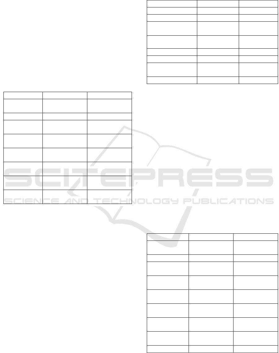
Table 3: Genetic Algorithm Calibration Results.
San Diego Andijan
Calibration
period
1960-1999 1934-2013
Best OSM 0.729724 0.072920
Diffusion/
derived
(90: 79-90)
100
(54:53-94)
82
Breed/ derived (23: 22-25)
26
(2:0-2)
3
Spread/ derived (89:74-98)
100
(88:62-94)
82
Slope/derived (13:2-32)
1
(70:9-70)
3
Road gravity/
derived
(19:19-98)
30
(47:14-47)
75
Calibration time
(s)
55588 19866
Speed Up 3.16 22.18
To investigate the spatial impact of the
differences in calibration mode, maps of forecast
Improving SLEUTH Calibration with a Genetic Algorithm
323
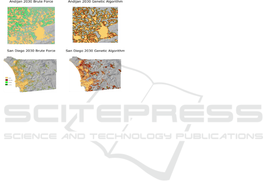
urbanization with a likelihood of over 50% were
created for the two cities and shown for both
methods of calibration (Figure 1). It is evident that
as in the calibrations, both cities are forecast with
higher uncertainty and greater spread using brute
force calibration, while the forecasts for both cities
are more constrained but with greater certainty using
GA. This appears to be the case both for high and
low model fit, and may be a robust way of providing
better forecasts.
Figure 1: Spatial extent of SLEUTH forecasts and Actual
Urban Growth During the Calibration Period.
4 CONCLUSION
Santé et al. (2010) pointed out the “need of making
urban CA more flexible while keeping their
simplicity by developing better calibration
methods.” This study has been in response to this
challenge. An important move, suggested by
Jafarnezhad et al. (2015) is to eliminate human
choices and judgements during the calibration
process, replacing the subjective with the objective
(Goldstein 2004). On the surface, replacing the brute
force calibration method for SLEUTH calibration
just substitutes a new set of calibration problems, i.e.
dealing with the characteristics of the gene and
determining how the evolutionary process yields the
best results. Prior work cited above, and now this
study, show that GA leads to at least equal, and
often superior calibration results while considerably
speeding the process. The results here also indicate
lower modeling uncertainty. The differences in the
calibration parameter sets are small, and the
differences among model forecasts are also small.
The advantages are the objectivity, and the benefits
of speed-up. At the least, GA can provide a
convergent set of genes that can be further optimized
by brute force over a much more limited parameter
set, such as the range over the top 8 genes listed in
table 3.
This study reviewed the importance of
calibration for CA land use change models.
Calibration performs important functions for models
because it ensures the model’s accuracy, integrity,
reliability and trustworthiness. Well calibrated
models are defensible and objective, and use real
world data instead of assumptions in their properties,
constants, variables and behavior types. There is an
obligation to perform sensitivity analyses and to run
controls. Moving SLEUTH calibration from brute
force to GA, the level of objectivity is further
improved. As a bonus, the amount of CPU time
devoted to calibration was reduced by about a factor
of 3 for San Diego and 22 for Andijan. Hopefully
this latter fact will enable new applications and new
cities to be simulated. The final version of the
SLEUTHGA software is posted at:
www.ncgia.ucsb.edu/projects/gig/Dnload/download.
htm and is available as open source code for
modelers.
REFERENCES
Blecic, I., Cecchini, A. and Trunfio, G. A. (2010) A
Comparison of Evolutionary Algorithms for
Automatic Calibration of Constrained Cellular
Automata. Taniar, D. et al. (Eds.): ICCSA 2010, LNCS
6016, 166–181. Springer-Verlag: Berlin.
Cao, K. Huang, B., Li, M. and Li, W. (2014) Calibrating a
cellular automata model for understanding rural–urban
land conversion: a Pareto front-based multiobjective
optimization approach, International Journal of
Geographical Information Science, 28:5, 1028-1046,
DOI: 10.1080/13658816.2013.851793
Cao, K., Wang, S., Li, X. and Chen, R. (2011) Modeling
Conversion of Rural-Urban Land Use Based on
Cellular Automata and Genetic Algorithm
Geoinformatics, 19th IEEE International Conference
on, Shanghai 1-5. DOI:
10.1109/GeoInformatics.2011.5981029
Clarke, K. C., Hoppen, S. and Gaydos, L. (1996) Methods
and Techniques for Rigorous Calibration of a Cellular
Automaton Model of Urban Growth. Proceedings, 3rd
Int. Conference/Workshop on Integrating GIS and
Environmental Modeling, January 21- 25th, Santa Fe,
NM.
Clarke, K. C., Hoppen, S. and L. Gaydos (1997) A self-
modifying cellular automaton model of historical
urbanization in the San Francisco Bay area.
Environment and Planning B: Planning and Design,
24, 247-261.
Clarke, K. C., and L. Gaydos (1998) Loose Coupling A
Cellular Automaton Model and GIS: Long-Term
GAMOLCS 2017 - International Workshop on Geomatic Approaches for Modelling Land Change Scenarios
324

Growth Prediction for San Francisco and
Washington/Baltimore. International Journal of
Geographical Information Science, 12, 7, 699-714.
Clarke, K.C. (2008a) Mapping and Modelling Land Use
Change: an Application of the SLEUTH Model, in
Landscape Analysis and Visualisation: Spatial Models
for Natural Resource Management and Planning,
(Eds. Pettit, C., Cartwright, W., Bishop, I., Lowell, K.,
Pullar, D. and Duncan, D.), Springer, Berlin, 353-366.
Clarke, K.C. (2008b) A Decade of Cellular Urban
Modeling with SLEUTH: Unresolved Issues and
Problems, Ch. 3 in Planning Support Systems for
Cities and Regions (Ed. Brail, R. K., Lincoln Institute
of Land Policy, Cambridge, MA, pp 47-60.
Clarke, K. C. (2014a) Why Simulate Cities? GeoJournal
79:129–136
Clarke, K. C. (2014b) Cellular Automata and Agent-Based
Models. Chapter 62 in Fischer, M. M. and Nijkamp, P.
(eds) Handbook of Regional Science. Springer-Verlag,
Berlin Heidelberg.
Clarke-Lauer, M. D., and Clarke, K. C. (2011). Evolving
simulation modeling: Calibrating SLEUTH using a
genetic algorithm. Proc., 11th Int. Conf. on Geo
Computation, Univ. College London, London.
Clarke, K. C. (in press) Land Use Change Modeling with
SLEUTH: Improving Calibration with a Genetic
Algorithm. In MT Camacho Olmedo, M Paegelow, JF
Mas, F Escobar (eds.) Geomatic approaches for
modelling land change scenarios . Lecture Notes in
Geoinformation and Cartography LNGC series.
Springer Verlag.
Chaudhuri, G. and Clarke, K. C. (2013) The SLEUTH
Land Use Change Model: A Review. Int. Journal of
Environmental Resources Research, 1, 1, 88-104.
Colonna, A., Di Stefano, V., Lombardo, S., Papini, L.,
Rabino, G. A. (1998). Learning urban cellular
automata in a real world: The case study of Rome
metropolitan area. In: ACRI’98 third conference on
cellular automata for research and industry, Trieste,
7–9 October 1998. London: Springer, 165–18.
Dietzel, C. and Clarke, K. C. (2007) Toward Optimal
Calibration of the SLEUTH Land Use Change Model.
Transactions in GIS, 11, 1, 29-45.
Feng, Y., Liu, Y., Tong, X., Liu, M., and Deng, S. (2011).
Modeling dynamic urban growth using cellular
automata and particle swarm optimization rules.
Landscape and Urban Planning, 102(3), 188–196.
http://dx.doi.org/10.1016/j.landurbplan.2011.04.004.
Feng, Y. and Liu, Y., 2012. An optimised cellular
automata model based on adaptive genetic algorithm
for urban growth simulation. In: W. Shi, A. Yeh, Y.
Leung and C. Zhou, eds. Advances in spatial data
handling and GIS: 14th international symposium on
spatial data handling. Heidelberg, Germany: Springer,
27–38.
García , A. M. I. Santé , M. Boullón and R. Crecente
(2013) Calibration of an urban cellular automaton
model by using statistical techniques and a genetic
algorithm. Application to a small urban settlement of
NW Spain, International Journal of Geographical
Information Science, 27:8, 1593-1611, DOI:
10.1080/13658816.2012.762454
Goldstein, N.C. (2004). Brains vs. Brawn: Comparative
strategies for the calibration of a cellular automata-
based urban growth model. In: P. Atkinson, G. Foody,
S. Darby and F. Wu, eds., GeoDynamics. Boca Raton,
FL: CRC Press.
Gong, Z., Tang, W., and Thill, J. C. (2012).
Parallelization of ensemble neural networks for spatial
land-use modeling. In Proceedings of the 5th ACM
SIGSPATIAL international workshop on location-
based social networks (pp. 48–54). ACM.
Guan, Q., Wang, L. and Clarke, K. C. (2005) An
Artificial-Neural-Network-based, Constrained CA
Model for Simulating Urban Growth . Cartography
and Geographic Information Science. 32, 4, 369-380.
Houet, T., Aguejdad, R., Doukari, O., Battaia G. and
Clarke, K. (2016) “Description and validation of a
‘non path-dependent’ model for projecting contrasting
urban growth futures”, Cybergeo : European Journal
of Geography, Systèmes, Modélisation,
Géostatistiques, document 759
http://cybergeo.revues.org/27397
Holland J. H. (1998). Emergence: From Chaos to Order.
Addison-Wesley, Redwood City, CA.
Hu, Z., and Lo, C. (2007). Modeling urban growth in
Atlanta using logistic regression. Computers,
Environment and Urban Systems, 31(6), 667–688.
Jafarnezhad, J., Salmanmahiny, A., and Sakieh, Y. (2015).
Subjectivity versus objectivity—Comparative study
between Brute Force method and Genetic Algorithm
for calibrating the SLEUTH urban growth model.
Urban Planning and Development.
doi:10.1061/(ASCE)UP.1943-5444.0000307.
Kirtland, D. Gaydos, L. Clarke, K. C., DeCola, L.,
Acevedo, W. and Bell, C. (1994) An analysis of
human-induced land transformations in the San
Francisco Bay/Sacramento area. World Resources
Review, 6, 2, 206-217.
Li, X. and Gar-On Yeh, A. (2002) Neural-network-based
cellular automata for simulating multiple land use
changes using GIS. International Journal of
Geographic Information Science. 16, 4, 323-343.
Li, X., and Yeh, A. G. O. (2004). Data mining of cellular
automata’s transition rules. International Journal of
Geographical Information Science, 18, 723–744.
Liu, Y., and Phinn, S. R. (2003). Modelling urban
development with cellular automata incorporating
fuzzy-set approaches. Computers, Environment, and
Urban Systems, 27, 637–658.
Long, Y., Mao, Q., and Dang, A. (2009). Beijing urban
development model: Urban growth analysis and
simulation. Tsinghua Science and Technology, 14(6),
782–794.
National Research Council (2014) Advancing Land
Change Modeling: Opportunities and Research
Requirements. Geographical Sciences Committee:
Washington D. C.; National Academy Press.
Pijanowski, B.C., B. Shellito and S. Pithadia. 2002. Using
artificial neural networks, geographic information
Improving SLEUTH Calibration with a Genetic Algorithm
325

systems and remote sensing to model urban sprawl in
coastal watersheds along eastern Lake Michigan.
Lakes and Reservoirs 7: 271-285.
Pontius Jr, R. G., W. Boersma, J-C. Castella, K. Clarke, T.
de Nijs, C. Dietzel, D. Zengqiang, E. Fotsing, N.
Goldstein, K. Kok, E. Koomen, C. D. Lippitt, W.
McConnell, A. M. Sood, B. Pijanowski, S. Pithadia, S.
Sweeney, T. N. Trung, A. T. Veldkamp, and P. H.
Verburg. (2007) Comparing the input, output, and
validation maps for several models of land change.
Annals of Regional Science, 42, 1 , 11-37.
Rienow, A. and Goetzke, R. (2014) “Supporting
SLEUTH—Enhancing a cellular with support vector
machines for urban growth modeling. Computers,
Environment and Urban Systems. 49, 66-81.
Sakieh, Y. (2013) Urban sustainability analysis through
the SLEUTH urban growth model and multi-criterion
evaluation. A case study of Karaj City. PhD
Dissertation, University of Tehran, Iran.
Santé, I., Garcia, A. M., Miranda, D. and Maseda, R. C.
(2010). Cellular automata models for the simulation of
real-world urban processes: a review and analysis.
Landscape and Urban Planning, 96 (2), 108–122.
Shan, J., Alkheder, S., and Wang, J., 2008. Genetic
algorithms for the calibration of cellular automata
urban growth modeling. Photogrammetric
Engineering and Remote Sensing, 74 (10), 1267–1277.
Silva, E.A. and Clarke, K.C. (2002) Calibration of the
SLEUTH urban growth model for Lisbon and Porto,
Portugal Computers, Environment and Urban Systems,
26, 6, 525-52 DOI 10.1016/S0198-9715(01)00014-X
Silva, E. A., and Clarke, K. C. (2005). “Complexity,
emergence and cellular urban models: Lessons learned
from applying SLEUTH to two Portuguese
metropolitan areas.” European Planning Studies,
13(1), 93–115.
Syphard, A. D., Clarke, K. C. Franklin, J., Regan, H. M.
and Mcginnis, M. (2011) Forecasts of habitat loss and
fragmentation due to urban growth are sensitive to
source of input data, Journal of Environmental
Management, 92, 7, 1882-1893.
Straatman, B., White, R., and Engelen, G., 2004. Towards
an automatic calibration procedure for constrained
cellular automata. Computers, Environment and
Urban Systems, 28, 149–170.
Torrens, P. T. and O’Sullivan, D (2001) Cellular automata
and urban simulation: where do we go from here?
Environment and Planning B: Planning and Design
28(2):163–168
Wu, F. and Webster, C. J. (1998) Simulation of land
development through the integration of cellular
automata and multi-criteria evaluation. Environment
and Planning B: Planning and Design 25(1):103–126
Wu, F. (2002) Calibration of stochastic cellular automata:
the application to rural-urban land conversions,
International Journal of Geographical Information
Science. 16 (8), 795–818.
Wu, X., Y. Hu, H. He, R. Bu, J. Onsted, and F. Xi (2009)
Performance Evaluation of the SLEUTH Model in the
Shenyang Metropolitan Area of Northeastern China
Environmental Modeling and Assessment 14, 2, 221-
230.
Xiang, W-N, and K. C. Clarke (2003) The use of scenarios
in land use planning. Environment and Planning B:
Planning and Design, 30, 885-909.
Yang, Q. S. and X. Li, (2007) Calibrating urban cellular
automata using genetic algorithms, Geographical
Research. 26, 2, 229–237.
Yang, Q., Li, X., and Shi, X. (2008). Cellular automata for
simulating land use changes based on support vector
machines. Computers and Geosciences, 34(6), 592–
602.
GAMOLCS 2017 - International Workshop on Geomatic Approaches for Modelling Land Change Scenarios
326
