B-kNN to Improve the Efficiency of kNN
Dhrgam AL Kafaf, Dae-Kyoo Kim and Lunjin Lu
Dept. of Computer Science & Engineering, Oakland University, Rochester, MI 48309, U.S.A.
Keywords:
Efficiency, kNN, k Nearest Neighbor.
Abstract:
The kNN algorithm typically relies on the exhaustive use of training datasets, which aggravates efficiency
on large datasets. In this paper, we present the B-kNN algorithm to improve the efficiency of kNN using a
two-fold preprocess scheme built upon the notion of minimum and maximum points and boundary subsets.
For a given training dataset, B-kNN first identifies classes and for each class, it further identifies the minimum
and maximum points (MMP) of the class. A given testing object is evaluated to the MMP of each class. If
the object belongs to the MMP, the object is predicted belonging to the class. If not, a boundary subset (BS)
is defined for each class. Then, BSs are fed into kNN for determining the class of the object. As BSs are
significantly smaller in size than their classes, the efficiency of kNN improves. We present two case studies
to evaluate B-kNN. The results show an average of 97% improvement in efficiency over kNN using the entire
training dataset, while making little sacrifice of the accuracy compared to kNN.
1 INTRODUCTION
The kNN algorithm (Cover and Hart, 1967) is widely
used for data classification in many application do-
mains (e.g., machine learning, data mining, bio-
informatics). kNN predicts the class of an object by
calculating the distance of the object to each sample
in the training dataset. Then, it predicts the class of
the object by the majority vote of its k neighbors.
However, considering every element in the training
dataset is expensive and erodes efficiency as the train-
ing dataset becomes larger, which is not suitable in the
real-time domain (e.g., automotive systems) where re-
sponse time is critical.
To address this, we present the B-kNN algorithm,
a variation of kNN equipped with a two-fold scheme
for preprocessing the training dataset to reduce the
size and improve the efficiency of kNN while mak-
ing little sacrifice of accuracy compared to kNN. The
two-fold preprocessing scheme is built upon the no-
tion of minimum and maximum points (MMP) and
boundary subsets (BS) of classes. Given a training
dataset, B-kNN identifies classes and for each class,
it further identifies its MMP which is the pair of the
minimum and maximum points of the class. For a
given testing object, B-kNN evaluates its belonging to
the MMP of each class. If there exists a class whose
MMP include the object, the object is predicted to be
of the class. If not, B-kNN defines the boundary sub-
set (BS) for each class which consists of the boundary
points of the class. Then, instead of the entire points
of classes, BSs are fed into kNN for predicting the
class of the object. BSs are significantly smaller in
size than their classes themselves and thus, the effi-
ciency of kNN significantly improves. Improved effi-
ciency is also contributed by avoiding repetitive pre-
processing on the entire training dataset when new
data is added. Only the new training data needs to
be processed. Furthermore, B-kNN addresses the
multi-peak distribution (Zhou et al., 2009) by adjust-
ing MMP to eliminate overlaps.
We conducted two case studies to evaluate B-
kNN. The results of the case studies show that B-kNN
improves an average of 97% in efficiency over kNN
using the entire training dataset with little sacrifice of
accuracy compare to kNN.
The remainder of the paper is organized as fol-
lows: Section 2 gives an overview of related work.
Section 3 describes the B-kNN algorithm. Section 4
presents the two case studies for evaluating B-kNN.
Section 5 concludes the paper with a discussion on
the future work.
2 RELATED WORK
Many researchers have studied methods for reducing
training datasets for classification in kNN to improve
efficiency.
126
Kafaf, D., Kim, D-K. and Lu, L.
B-kNN to Improve the Efficiency of kNN.
DOI: 10.5220/0006393301260132
In Proceedings of the 6th International Conference on Data Science, Technology and Applications (DATA 2017), pages 126-132
ISBN: 978-989-758-255-4
Copyright © 2017 by SCITEPRESS – Science and Technology Publications, Lda. All rights reserved

In text classification (Zhou et al., 2009) pre-
sented a modified kNN algorithm to preprocess train-
ing datasets using the k-mean clustering algorithm
(MacQueen et al., 1967) to find the centroid of each
known class. After identifying the centroid, the algo-
rithm eliminates far-most points in the class to avoid
the multi-peak distribution effect which involves mul-
tiple classes overlapping. After the elimination, the
k-mean clustering algorithm is used to identify sub-
classes and their centroids which forms a new training
dataset.
(Muja and Lowe, 2014) presented a scalable kNN
algorithm to reduce the computation time for a large
training dataset by clustering the dataset to N clusters
and distributing them to N machines where each ma-
chine is assigned an equal amount of data to process.
The master server distributes the query for a testing
data to predict its class so that each machine can per-
form the kNN algorithm execution in parallel and re-
turn the results to the master server for consolidation.
(Xu et al., 2013) presents the coarse to fine kNN
classifier which is a variation of kNN using a recur-
sive process for refining a triangular mesh which rep-
resents a subset of the training dataset. As the trian-
gulation of the mesh is refined, the size of the subset
is reduced.
(Parvin et al., 2008) present a modified weighted
kNN algorithm to enhance the performance of kNN.
The algorithm preprocesses the training dataset using
the testing dataset. The preprocessing first determines
the validity of each data point by measuring its sim-
ilarity to its k neighbors and then measures its dis-
tance weight to each data point in the testing dataset.
The product of the validity and distance weight for
each data point produces a weighted training dataset.
This reduces a multi-dimensional dataset into one-
dimensional dataset, which improves the efficiency of
kNN.
(Lin et al., 2015) combine the kNN algorithm
with the k-mean clustering algorithm to improve the
accuracy and efficiency of kNN for intrusion detec-
tion by preprocessing the training dataset. The pre-
processing involves finding the centroid of each class
using the k-mean clustering and computing the dis-
tance between each point in the class to its neigh-
bors and the class centroid. The same preprocess-
ing applies to the testing dataset. Similar to Parvin
et al.’s work, it can be considered as converting the
n-dimensional dataset into one-dimensional dataset.
(Yu et al., 2001) introduce a distance-based kNN
algorithm to improve the efficiency of kNN by pre-
processing the training dataset. The preprocessing in-
volves partitioning the training dataset and identifying
the centroid of each partition to be a reference point to
the partition. Then, they compute the distance of each
data point in the partition to the reference point and
index the distances in a B
+
tree. For a testing data,
the closest partition is found by computing the dis-
tance of the data to the centroids of partitions. Once
the closet partition is identified, the B
+
tree of the par-
tition is used to search the nearest neighbor to the data
in the partition.
In summary, the existing work involves a certain
type of preprocessing of training datasets to improve
the efficiency of kNN. The preprocessing in the ex-
isting work is repetitive on the entire training dataset
when the training dataset is updated, which involves
significant overheads. However, the B-kNN algo-
rithm presented in this work requires only the new
training data to be preprocessed rather than the entire
training dataset.
3 B-KNN
In this section, we describe the B-kNN algorithm to
improve efficiency. B-kNN enhances the efficiency
of the traditional kNN algorithm by reducing compu-
tation time through preprocessing the training dataset.
Figure 1 shows an overview of the B-kNN algorithm
approach. It consists of two activities – (i) prepro-
cessing the training dataset to define the minimum
and maximum points (MMP) and the boundary subset
(BS) of the class and (ii) predicting the type of a test-
ing object using the minimum and maximum points
and the boundary of classes.
Training
Dataset
Separate Classes
Define MMP of
Class
Data Within MMP
kNN
Tes"ng
Dataset
Data
Classified
Y
N
MMP
Define BS of Class BS
Preprocessing
Predic"on
Figure 1: B-kNN algorithm overview diagram.
3.1 Preprocessing Training Dataset
A given training dataset contains data elements which
are defined in terms of attributes. Data elements are
grouped by the value of the designated attribute that
is used to classify a given testing dataset. Classes can
be projected onto a multi-dimensional plot per the at-
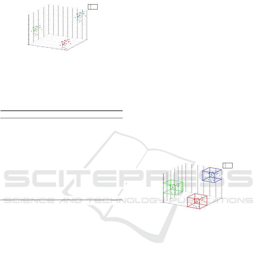
tributes of their constituent elements. Figure 2 shows
an example of a three-dimensional plot that involves
three classes whose elements have three attributes.
B-kNN to Improve the Efficiency of kNN
127

1
2
3
4
5
0
0.5
1
1.5
2
2.5
3
3.5
4
1
1.5
2
2.5
3
3.5
4
X
Y
Z
Class 1
Class 2
Class 3
Figure 2: Classes distribution.
Algorithm 1 describes defining classes by the
value of the designated attributes and storing them
into lists. For each class, the preprocessing of B-kNN
defines its MMP and BS which are used to predict the
class of a testing element.
Algorithm 1: Class separation.
1: procedure SEPARATE CLASSES(td: in Train-
ing Dataset, ct: out Class Type, cd: out Class
Dataset)
2: for each instance in td, do
3: if instance label ∈ ct then
4: class dataset ← instance
5: else
6: ct ← instance label
7: cd ← instance
8: end if
9: end for
10: end procedure
Defining MMP. The MMP of a class are de-
termined by the minimum and maximum value
of each dimension (attribute) of the class. For a
non-numerical attribute, the value is converted to a
numerical value. For example, consider a class
C
1
={(Red,1,6),(Blue,5,7),(Green,7,8),(Yellow,9,3),
(Black,2,10)}
The first-dimension of the class is non-numerical,
and thus needs to be converted to a numerical value
as follows. Red → 1, Blue → 2, Green → 3, Yellow
→ 4, and Black → 5. Per the mapping, the training
dataset becomes
C
1
={(1,1,6),(2,5,7),(3,7,8),(4,9,3),(5,2,10)}
Part of the data preprocessing is to remove out-
liers. An outlier is an observation point that is distant
from other observations. An outlier makes MMP
wider which distorts the prediction and thus reduces
accuracy. In the set, the minimum value is 1 for the
first dimension, and 1 for the second dimension, and
3 for the third dimension. Thus, the minimum point
is defined as C
1
min
={(1,1,3)}. The maximum point
is defined similarly as C
1
max
={(5,9,10)}. The MMP
is then used for determining the class of a testing
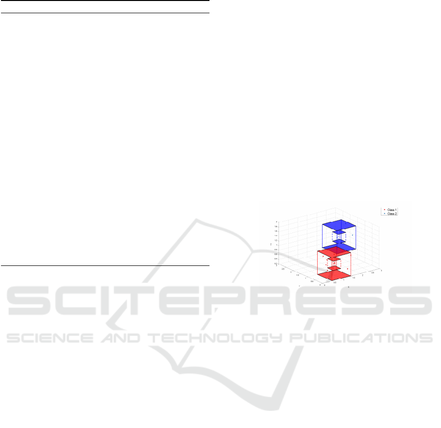
element. Figure 3 shows the cubes determined by
the MMPs of the classes in Figure 2 If the testing
element does not fall into the range of the MMP, we
use the BS of the class as a secondary method for
determining the class.
Defining BS. We define the BS of a class by se-
lecting the points that have either minimum or max-
imum value of any dimension. For example, in
C
1
, (1,1,6) has its first and second dimension min-
imum, (4,9,3) has its second dimension maximum,
and (5,2,10) has its first dimension and third dimen-
sion maximum. Thus, the BS of C
1
is identified as
C
1
BS
={(1,1,6),(4,9,3),(5,2,10)} which is a subset of
the class. Then, for each point in the boundary, its dis-
tance to the testing object is measured and the shortest
distance becomes the distance of the testing element
to the class. Note that we use Euclidean distance in
this work.
1
1.5
2
2.5
3
3.5
4
0
0.5
1
1.5
2
2.5
3
1
1.5
2
2.5
3
3.5
4
X
Y
Z
Class 1
Class 2
Class 3
Figure 3: Class boundaries.
Given C
1
BS
, suppose a testing element
T
1
=(6,10,2). Then, the distance of T
1
to the in-
dividual elements of the BS is measured as 11.045
to (1,1,6), 2.449 to (4,9,3), and 11.357 to (5,2,10).
Thus, the distance of T
1
to C
1
is determined as
the shortest distance T
1
C1
=2.449. We measure the
distance to every class and use the shortage distance
to determine the class of the given testing element.
This improves the efficiency of prediction by using
the subset rather than the entire training dataset.
Algorithm 2 describes defining the MMP and BS of
a class.
3.2 Predicting Testing Dataset
The class of a testing element is predicted based on
the minimum and maximum points of classes and its
distance to classes defined in Subsection 3.1. First,
the testing element is evaluated if it is within the range
DATA 2017 - 6th International Conference on Data Science, Technology and Applications
128

Algorithm 2: MMP and BS.
1: procedure FIND MAX POINT(cd: in Class
Dataset, BS: out Boundary Subset, CMAX: out
Class Maximum Point)
2: for each instance in cd do
3: if instance > maxInstance then
4: maxInstance ← instance
5: end if
6: end for
7: CMAX ← maxInstance
8: BS ← [instance ∈ maxInstance]
9: end procedure
10: procedure FIND MIN POINT (cd: in Class
Dataset, BS: out Boundary Subset, CMIN: out
Class Minimum Point)
11: for each instance in cd do
12: if instance < minInstance then
13: minInstance ← instance
14: end if
15: end for
16: CMIN ← minInstance
17: BS ← [instance ∈ minInstance]
18: end procedure
the MMP of a class. If so, the testing element is
predicted belonging to the class. For example, con-
sider a testing data T
2
={(2,8,4)}. Per C
1
min
={(1,1,3)}
and C
1
max
={(5,9,10)} of C
1
, T
2
is within the range of
the MMP, and thus it is predicted belonging to C
1
.
Suppose anther class
C
2
={(11,19,18),(10,26,17),(25,25,19),
(29,17,18),(31,12,20)}
The MMP of C
2
is identified as C
2
min
=(10,12,17) and
C
2
max
=(31,26,20) respectively. Also, the BS of C
2
is
identified as
C
2
BS
={(10,26,17),(31,12,20)}
Consider T
1
again. It is out of the range of the
MMP of both C
1
and C
2
and the class of T
1
cannot
be predicted by the MMP of C
1
and C
2
. In such a
case, the shortest distance of T
1
to C
1
and C
2
is used
to predict the class of T
1
. The distance of T
1
to C
1
is measured as T
1
C1
=2.449 in Subsection 3.1. For
C
2
, the distance of T
1
to the BS of C
2
is measured
as 22.293 for (10,26,17) and 30.870 for (31,12,20).
Thus, the distance of T
1
to C
2
is measured as 22.293.
This is far greater than the distance to C
1
, which
means that T
1
is closer to C
1
. Therefore, T
1
is
predicted belonging to C
1
. After the inclusion of T
1
in C
1
, the BS of C
1
is updated as
C
1
BS
={(1,1,6),(6,10,2),(5,2,10)}
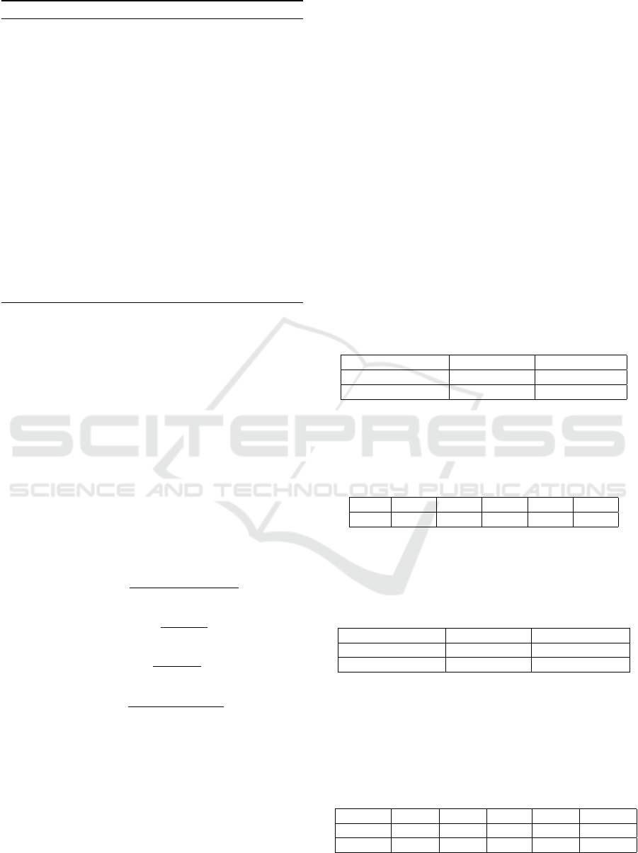
Note that classes may overlap in which case the
accuracy of classification decreases if the testing
element is in the overlap. This is known as multi-peak
distribution. Consider
C
3
={(1,1),(2,2),(1,16),(10,1),(10,15),(12,1),(12,16)}
C
4
={(10,2),(13,3),(13,17),(10,18),(19,17),(20,2),
(20,18)}
the MMP of C
3
and C
4
are defined as C
3
min
=(1,1) and
C
3
max
=(12,16) and C
4
min
=(10,2) and C
4
max
=(20,18)
where C
3
max
overlaps with C
4
min
. Therefore, a testing
data T
3
=(11,9) is identified as being in the over-
lap. Figure 4 illustrates an example of multi-peak
distribution.
Figure 4: Multi-peak distribution.
In the case of multi-peak distribution, we ad-
just the MMP of the overlapping classes to elimi-
nate the overlap by identifying the next smallest min-
imum point and the next largest maximum point. In
the above example, the MMP of C
3
is adjusted as
C
3
min
=(2,2) and C
3
max
=(10,15) and the MMP of C
4
is
adjusted as C
4
min
=(13,3) and C
4
max
=(19,17). After the
adjustment, there is no overlap between C
3
and C
4
,
and thus T
3
no longer resides in any overlap. Now,
we measure the distance of T
3
to C
3
and C
4
which
is measured as 6.08 and 6.32 respectively. Thus, T
3
is predicted belonging to C
3
. The same technique
is used when more than two classes are overlapped.
Although the MMP boundaries are reduced, the BS
points of classes remain the same. If a testing point
falls outside the MMP, the traditional kNN algorithm
is used for prediction using the BS points of classes.
Algorithm 3 describes the classification process. The
algorithm starts with training kNN using the BSs of
the training dataset. Then, the testing dataset is evalu-
ated to the MMP of each class in the training dataset.
If the testing data falls within the MMP, the class type
is added to the prediction list. If not, kNN is per-
formed and the prediction is added to the prediction
list.
B-kNN to Improve the Efficiency of kNN
129

Algorithm 3: Prediction and evaluation.
1: procedure PREDICTION(BS: in Boundary Sub-
set, CMAX: in Class Maximum Point, CMIN: in
Class Minimum Point, pl: out Predictions List,
el: out Evaluation List)
2: initialize kNN(BS)
3: for each class do
4: for each instance in testing dataset do
5: if instance ≤ CMAX and instance ≥
CMIN then
6: pl ← classtype
7: else
8: pl ← kNN.classify(instance)
9: end if
10: end for
11: end for
12: el ← evaluate(predictions list)
13: end procedure
4 VALIDATION
To validate the B-kNN algorithm, we conducted two
case studies. One case uses datasets in the context
of room properties (e.g., temperature, occupancy) and
the other case uses datasets in the context of personal
information (e.g., age, salary). We apply the B-kNN
algorithm to the case studies and measure its accu-
racy, recall, precision, and F1 score using confusion
matrices (Townsend, 1971) which represent the per-
formance of a classification model in terms of true
positive, true negative, false positive, and false nega-
tive.
Accuracy =
T P + T N
T P + FP + FN + T N
(1)
Precision =
T P
T P + FP
(2)
Recall =
T P
T P + FN
(3)
F1 = 2 ∗
Precision ∗ Recall
Precision + Recall
(4)
We implemented the B-kNN algorithm using Java
JDK 8 and WEKA (Hall et al., 2009), a data min-
ing application, on Intel Pentium Quad-Core Proces-
sor with 3.40GHz and 8GB of memory.
4.1 Case Study 1
In this study, we use the datasets used in the work by
Candanedo and Feldheim (Candanedo and Feldheim,
2016) which contain data collected from room sen-
sors monitoring temperature, humidity, light, CO2,
humidity ratio, and occupancy. These factors consti-
tute the attributes of data. The training dataset con-
tains 8143 data elements which are used to classify
a testing dataset of 2665 data elements. There is no
missing data in both the training and testing datasets.
The study was carried out comparatively by com-
paring the results of applying the traditional kNN al-
gorithm to the original training dataset with the results
of by applying the B-kNN algorithm to the MMP and
BS of the original training dataset. This study is con-
cerned with predicting the occupancy of the room in
the testing dataset. Table 1 shows the results of the
former represented in a confusion matrix. The ta-
ble shows 854 instances correctly predicted and 55
instances falsely predicted as the room is occupied.
On the other hand, 118 instances are falsely predicted
and 1638 instances are correctly predicted as the room
was not occupied.
Table 1: Confusion matrix for kNN.
Room Occupancy Occu. (Pred.) Unocc. (Pred.)
Occu. (Act.) 854 118
Unoccu. (Act.) 55 1,638
Table 2 shows the accuracy, precision, recall, F1,
response time (in second) of the kNN algorithm on
the confusion matrices in Table 1.
Table 2: Results of kNN.
Alg. Acc. Prec. Rec. F1 Time
kNN 0.935 0.939 0.879 0.908 1.254
Table 3 shows the confusion matrix of the B-kNN
algorithm applying to the MMP and BS of the training
dataset.
Table 3: Confusion matrix for B-kNN.
Room Occupancy Occu. (Pred.) Unoccu. (Pred.)
Occu. (Act.) 838 104
Unoccu. (Act.) 71 1,652
Table 4 shows the results of the B-kNN algorithm
on the confusion matrices in Table 3. The table shows
a slight decrease on accuracy, precision, and F1 and a
slight improvement on recall. On the other hand, the
response time is improved significantly by 94.7%.
Table 4: Results of B-kNN.
Alg. Acc. Prec. Rec. F1 Time
B-kNN 0.934 0.922 0.889 0.905 0.066
Improv. -0.1% -1.8% 1.1% -0.3% +94.7%
DATA 2017 - 6th International Conference on Data Science, Technology and Applications
130

4.2 Case Study 2
In this study, we use the dataset from Lichman’s
repository (Lichman, 2013) which contains personal
information of age, work class, final weight, edu-
cation, marital-status, occupation, relationship, race,
gender, capital gain, capital loss, working hours per
week, native country, and whether the salary is over
50K or not. The training dataset contains 32,561 data
elements which are used to classify the testing dataset
of 16,281 data elements. The B-kNN algorithm is
used to predict whether the person in a testing data
makes over 50K in salary. There is no missing data in
both the training and testing datasets.
Table 5 shows the confusion matrix of applying
the traditional kNN algorithm to the original training
dataset. The table shows that 10,625 instances are
correctly predicted as the person’s salary over 50K,
while 594 instances are falsely predicted. On the
other hand, 1,165 instances are falsely predicted as
the person’s salary under 50K, while 3,897 instances
are correctly predicted.
Table 5: Confusion Matrix for kNN.
Salary ↑ 50K (Pred.) ↓ 50K (Pred.)
↑ 50K(Act.) 10,625 1,165
↓ 50K (Act.) 594 3,897
Table 6 shows the accuracy, precision, recall, F1,
response time (in second) of the kNN algorithm on
the confusion matrices in Table 5.
Table 6: Results of kNN.
Alg. Acc. Prec. Rec. F1 Time
kNN 0.892 0.947 0.901 0.924 26.797
Table 7 shows the confusion matrix of applying
the B-kNN algorithm to the MMP and BS of the train-
ing dataset.
Table 7: Confusion Matrix for B-kNN.
Salary ↑ 50K (Pred.) ↓ 50K (Pred.)
↑ 50K(Act.) 10,563 1,083
↓ 50K (Act.) 656 3,979
Table 8 shows the results of the B-kNN algorithm
on the confusion matrix in Table 7. Similar to the
observation made in Table 4, we can observe that the
accuracy, precision, recall, and F1 are very close to
those of the kNN algorithm in Table 6. However, the
response time is significantly improved by 99.3%.
Table 8: Results of B-kNN.
Alg. Acc. Prec. Rec. F1 Time
B-kNN 0.893 0.942 0.907 0.924 0.194
Improv. +0.1% -0.5% +0.6% 0.0% +99.3%
4.3 Discussion
As seen in the two case studies, the B-kNN algorithm
gives a similar performance on accuracy, precision,
recall, and F1. However, it dramatically improves re-
sponse time by 97% in average. This becomes more
significant for larger datasets. We used the value 1 for
k in the kNN algorithm in the case studies. We also
experimented higher values for k up to 7. In Case
Study 1, the accuracy and response time of kNN us-
ing the original training dataset are slightly improved
(less than 1%), while B-kNN remains more or less
the same. In Case Study 2, the accuracy of kNN de-
creases about 11 % at k=2 and becomes stabilizes
since then. Similarly, the response time of kNN in-
creases about 35% in average since k=2. However,
the accuracy and the response time of B-kNN remains
stable as in Case Study 1. The different results in the
two studies are attributed to the size of the training
dataset of Case Study 2 being much larger than that
in Case Study 1. The experiments show that B-kNN
gives stable results for higher k values compared to
kNN using the original training dataset. This benefit
becomes significant for larger datasets as shown in the
two case studies.
5 CONCLUSION
We have presented the B-kNN algorithm to improve
the efficiency of the traditional kNN, while maintain-
ing similar performance on accuracy, precision, re-
call, and F1. The improvement is attributed to the
two-fold preprocessing scheme using the MMP and
BS of training datasets. B-kNN also addresses the de-
fect of uneven distributions of training samples which
may cause the multi-peak effect by updating the BS
as a new training sample is added. The two case stud-
ies presented in this paper validate the B-kNN algo-
rithm by demonstrating its improvement on efficiency
over the kNN algorithm. The results show a signifi-
cant enhancement in efficiency with little sacrifice of
accuracy compared to the traditional kNN algorithm.
In the future work, we plan to apply the B-kNN algo-
rithm to self-adaptive systems in the robotic domain
to enhance response time which is crucial for self-
adaptive operations.
B-kNN to Improve the Efficiency of kNN
131

REFERENCES
Candanedo, L. M. and Feldheim, V. (2016). Accurate Occu-
pancy Detection of an Office Room from Light, Tem-
perature, Humidity and CO 2 Measurements Using
Statistical Learning Models. Energy and Buildings,
112:28–39.
Cover, T. and Hart, P. (1967). Nearest Neighbor Pat-
tern Classification. IEEE Transactions on Information
Theory, 13:21–27.
Hall, M., Frank, E., Holmes, G., Pfahringer, B., Reutemann,
P., and Witten, I. H. (2009). The WEKA Data Mining
Software: an Update. ACM SIGKDD Explorations
Newsletter, 11(1):10–18.
Lichman, M. (2013). UCI machine learning repository.
Lin, W.-C., Ke, S.-W., and Tsai, C.-F. (2015). CANN:
An Intrusion Detection System Based on Combining
Cluster Centers and Nearest Neighbors. Knowledge-
Based Systems, 78:13–21.
MacQueen, J. et al. (1967). Some Methods for Classi-
fication and Analysis of Multivariate Observations.
In Proceedings of the Fifth Berkeley Symposium on
Mathematical Statistics and Probability, volume 1,
pages 281–297. Oakland, CA, USA.
Muja, M. and Lowe, D. G. (2014). Scalable Nearest Neigh-
bor Algorithms for high Dimensional Data. IEEE
Transactions on Pattern Analysis and Machine Intel-
ligence, 36(11):2227–2240.
Parvin, H., Alizadeh, H., and Minaei-Bidgoli, B. (2008).
MKNN: Modified K-Nearest Neighbor. In Proceed-
ings of the World Congress on Engineering and Com-
puter Science, volume 1. Citeseer.
Townsend, J. T. (1971). Theoretical Analysis of an Alpha-
betic Confusion Matrix. Perception & Psychophysics,
9(1):40–50.
Xu, Y., Zhu, Q., Fan, Z., Qiu, M., Chen, Y., and Liu, H.
(2013). Coarse to Fine K Nearest Neighbor Classifier.
Pattern Recognition Letters, 34(9):980–986.
Yu, C., Ooi, B. C., Tan, K.-L., and Jagadish, H. (2001).
Indexing the Distance: An Efficient Method to Knn
Processing. In VLDB, volume 1, pages 421–430.
Zhou, Y., Li, Y., and Xia, S. (2009). An Improved KNN
Text Classification Algorithm Based on Clustering.
Journal of Computers, 4(3):230–237.
DATA 2017 - 6th International Conference on Data Science, Technology and Applications
132