Realistic Estimation of Model Parameters

Pavel Ettler

COMPUREG Plzeˇn, s.r.o., 306 34, Plze´n, Czech Republic

Keywords:

Parameter Estimation, Process Model, Probabilistic Distribution, Adaptive Control.

Abstract:

Most often, the normal distribution N plays the key role in the process modelling and parameter estimation.

The paper deals with realistic estimation of model parameters which takes into account limitations on pa-

rameters which arise in industrial applications of the model-based adaptive control. Here the limitation of

a normally distributed random variable is being modelled by speciﬁc distribution – the probabilistic mixture

D. It is shown that relationship between distributions N and D coincides with properties of the generalized

normal distribution G and that relations between their ﬁrst and second statistical moments can be adequately

approximated by G’s cumulative distribution function and probability density function, respectively. The de-

rived method is then applied to estimation of bounded parameters. In combination with the idea of parallel

identiﬁcation of the full and reduced models of the process, a working algorithm is derived. Performance of

the algorithm is illustrated by examples on both simulated and real data.

1 INTRODUCTION

The notion of adaptive control ﬁrst appeared already

in the ﬁfties of the last century – see, e.g. (

Astr¨om

and Kumar, 2014) for further references. Its boom

started in the seventies with the expectation of broad

utilization of the adaptive control not only in the in-

dustrial practice. Presently, this type of control has

found its place in real applications but in the extent

far from earlier assumption. Among reasons of such

progress and today’s situation there is one that orig-

inates in the mismatch between the process model

and the real system or more likely, in disrespecting

such discrepancy which always exists in practice. It

is closely connected with the fact that measured data

which are available for the model and estimation of

its parameters are always burdened with uncertainty.

Searching for a model which preferably approx-

imates behaviour of the observed or even controlled

system in all situations and handling of every conceiv-

able exceptions turned out to be so demanding and

time-consuming that other types of control, PID con-

trol in particular, dominate the scene regarding num-

ber of applications. In effect, the model-based adap-

tive control is being employed just in cases where in-

creased demands on its implementation pay off and

when the search for a model based on the imperfect

data leads to an acceptable result.

It proves that the model-based control is facing the

problem which is inherent also for other theoretical

approaches to control: if we are “inside” the elabo-

rated theory everything ﬁts together and all tasks seem

solvable. The problem occurs on the boundary of the

given theory and real world – the reality does not re-

spect prerequisites of the approach, the model is just

approximation of the real system, data are corrupted

by noise or burdened by uncertainty in general.

The aim of the paper is to contribute usefully to

solution of the problem in the borderland between

theory and reality.

1.1 Bounded Parameter Estimation

Bounded estimation issues are anything but new and

motivation for the solution exists in many application

ﬁelds which corresponds to the variedness of journals

and proceedings in which at least partial solutions are

being published. Nevertheless, it has been observed

(Murakami and Seborg, 2000; Kopylev, 2012) that

very few thorough monographs exist in this respect

(Van Eeden, 2006).

1.2 Existing Variety of Solutions

As the result, state of affairs is rather disorganized

but even so, the solutions can be divided by the type

of limitation being applied (with citation examples in

brackets):

• Limitation on the estimation error (Milaneseet al.,

1996),

• Limitation on the system noise (Norton, 1987),

• Conﬁdence intervals (Mandelkern, 2002),

Ettler, P.

Realistic Estimation of Model Parameters.

DOI: 10.5220/0006395705270534

In Proceedings of the 14th International Conference on Informatics in Control, Automation and Robotics (ICINCO 2017) - Volume 1, pages 527-534

ISBN: 978-989-758-263-9

527

• Statistically bounded (soft-constrained) estima-

tion (Benavoli et al., 2006),

• Sharp restrictions on the parameter estimates

(K´arn´y, 1982; Benavoli et al., 2006; Ettler and

K´arn´y, 2010).

The presented solution belongs to the latter type.

2 PROCESS MODEL AND ITS

PARAMETERS

Consider a process model for which X

= [y(t),z(t)]

stand for vector of observations, where the output y

is in discrete time instants t = 1,2,. .. related to mea-

sured data

z(t) = [y(t − 1), ... , y(t − m

), (1)

= u

(t), ... , u

(t − m

= v(t), ..., v(t − m

),1]

Vector z is composed by m

samples of past

outputs y, m

+ 1 samples of controllable inputs u

and m

+ 1 samples of measurable disturbances v.

System output y is here considered as scalar for the

sake of simplicity, while inputs and disturbances

can be multidimensional. Number one as the last

vector element enables to consider an absolute term

alias offset. The considered stochastic relation is

parameterized by unknown parameters Θ with ﬁnite

dimension and can be described by the probability

density function (pdf) f(y| z,Θ).

Note: Most of the discussed variables are considered

to be time-variant. Nevertheless, the time index is

sometimes omitted in the following text for the sake

of simplicity.

2.1 Linear Gaussian Model

In practice, the linear regression model is mostly con-

sidered and the uncertainty is approximated by the

normal (Gaussian) probability distribution N deﬁned

by two parameters

f(y|z,Θ) = N (ˆy,σ

) , (2)

where ˆy(t) = θ

′

(t)z(t) and

Θ = [θ, σ

] (3)

are unknown parameters of the system,

while θ = [ϑ

, ϑ

, ... , ϑ

]

′

, m = m

+ (m

+ 1) +

+ 1)+ 1 and σ

stands for the variance of the sys-

tem noise. Equivalently, the model can be expressed

y(t) = θ

′

(t)z(t)+ e(t) (4)

with the system noise e(t) ∼ N (0,σ

2.2 Estimator of Unknown Parameters

Author’s regular choice regarding parameter estima-

tion is Bayesian probabilistic approach. Here un-

known parameters can be considered to be random

variables described by the pdf f(Θ| y,z). It can be

derived (Peterka, 1981; K´arn´y et al., 2005)) that for

the model (4) and ﬁxed parameters the pdf is fully

speciﬁed by the positive deﬁnite information matrix

V which – after introduction of some type of forget-

ting (Kulhav´y and Zarrop, 1993) to allow tracking of

varying parameters – can be recursively updated as

V(t) = ϕV(t − 1) + [y(t),z(t)]

′

[y(t), z(t)], (5)

where ϕ ∈ (0,1i is forgetting factor. Partitioning of V

V =



′



(6)

enables to express the parameter estimates

θ = V

−1

. (7)

Variances of system noise and parameter estimates,

respectively, can be estimated as

−V

′

−1

, (8)

diag(V

−1

) , (9)

where

κ(t) = ϕκ(t − 1) + 1 . (10)

In real-time applications it is appropriate to work with

V in its factorized form V

−1

= LDL

′

(Peterka, 1981)

for the sake of numerical stability.

3 RESPECTING LIMITATIONS

OF REAL-LIFE QUANTITIES

Even if unlimited quantities exist in the real world,

our observations of them are always bounded. Find-

ings of consideration about an observed general

bounded variable will be used for the parameter es-

timates in the following sections.

3.1 Probabilistic Formulation of

Limitation

Consider a real-world variable ξ and its observation x

in discrete time instants t = 0,1,.... The observation

is bounded by x

= x

min

a x = x

max

which are given e.g.

by a sensor range. Then it holds

x(t) =







for ξ(t) ≤ x

ξ(t) for ξ(t) ∈ (x, x)

x for ξ(t) ≥ x .

(11)

ICINCO 2017 - 14th International Conference on Informatics in Control, Automation and Robotics

528

Let ξ be considered a normally distributed random

variable ξ ∼ N (µ

,σ

). Owing to the limitation (11),

distribution of x is not Gaussian but can be expressed

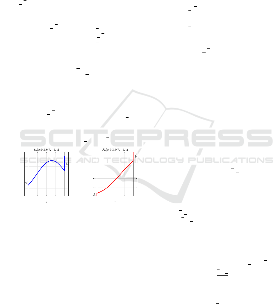
by a probabilistic mixture D the pdf of which is

composed by a central part of normal pdf and two

Dirac functions δ at boundary points of the interval

,xi (Benavoli et al., 2006).

Then, the pdf of D is represented by

(x|µ

,σ

,x) = Aδ(|ξ− x|) + (12)

(ξ ∈ hx

,xi|µ

,σ

) +

Bδ(|ξ−

x|) ,

where

A = F

|µ

,σ

) (13)

B = 1− F

(

x|µ

,σ

) , (14)

where F

stands for cumulative distribution function

(cdf) of normal distribution and cdf of D reads

(x|µ

,σ

,x) =







0 for ξ < x

(ξ|µ

,σ

) for ξ ∈ hx,xi

1 for ξ > x .

(15)

Example in Fig. 1 shows pdf and cdf of D with pa-

rameters µ

= 0.3, σ

= 0.7, x = −1 a x = 1.

-1 -0.5 0 0.5 1

0.1

0.2

0.3

0.4

0.5

-1 -0.5 0 0.5 1

0.2

0.4

0.6

0.8

Figure 1: Pdf and cdf of the probabilistic mixture D.

3.2 Distribution D and Parameter

Estimation

Obviously, properties of the normal distribution N

which make it exceptionally suitable for estimation

algorithm development cannot be expected in the het-

erogenous distribution D.

Exact solution can be found only in the case of one

bounded parameter (Benavoli et al., 2006). General

case leads to utilization of iterative numerical meth-

ods which are not very suitable for real-time applica-

tions. It is necessary to look for another solution.

3.3 Relations between Statistical

Moments of Distributions N and D

As a consequence of (11), mean values µ

, µ

and

variances σ

, σ

will differ while it holds

∈ hx

, xi,







> µ

for µ

< M

= µ

for µ

= M

< µ

for µ

> M







(16)

M = (x

+ x)/2 (17)

∈ h0, σ

i . (18)

In the case of success to evaluate relation

{µ

,σ

,x} → {µ

⋆

,σ

2⋆

} , (19)

while respecting conditions (17) and (18), it would be

possible to apply the rule for calculation of bounded

parameter estimates Θ.

3.4 Employment of the Generalized

Normal Distribution G

Extensive experiments led to the result that relations

between variances σ

and σ

of distributions N and

D can be successfully approximated by the pdf of the

generalized normal distribution G and relations be-

tween means µ

and µ

can be approximated by cdf

of the same distribution (see Appendix for properties

of distribution G).

Simple rules were found for computation of G’s

parameters µ

, α and β:

: For the allowable range x ∈ h

x, xi, it is natural to

place the mean µ

in the middle M (17) of the

interval.

α: It is possible to deﬁne width of the distribution G

as a distance between inﬂection points of its pdf

while these points coincide with limits of the in-

terval h

x,xi. Then, parameter α can be expressed

as α = (x− x)/2.

β: Experiments have shown that the shape of f

re-

mains the same for constant ratio of the interval

span (i.e. of parameter α) to the standard devia-

tion σ

. Therefore the shape parameter β can be

deﬁned as β = α/σ

To sum up, following relations hold for x

= 0, x = 1

and σ

= 1:

α =

x− x

(20a)

β =

(20b)

= x

+ α (20c)

Modiﬁcation of equations (20) for general case is

described below.

Realistic Estimation of Model Parameters

529

3.5 Limiting Functions ℓ

, ℓ

As was already mentioned, group of equations (20)

allows to construct f

and F

which approximate re-

lationship between unboundedand bounded moments

for the special case (x

= 0, x = 1, σ

= 1).

Let call the limiting functions for both moments

ℓ

, ℓ

. Following restrictive conditions enabled to

ﬁnd formulation of the functions for general values of

boundaries x

, x and variance σ

min

∈R

ℓ

(µ

|σ

,x) = x (21a)

max

∈R

ℓ

(µ

|σ

,x) = x (21b)

min

∈R

ℓ

(µ

|σ

,x) = 0 (21c)

max

∈R

ℓ

(µ

|σ

,x) = σ

(21d)

While f

is a non-negative symmetrical function,

its maximum lies in the middle µ

(20c) of the bound-

ing interval; therefore it holds for extreme values of

G,min

= 0 (22a)

G,max

= f

(µ

|µ

,α,β) . (22b)

As F

represents cdf it holds

G,min

= F

(ξ

−∞

|µ

,α,β) = 0 (23a)

G,max

= F

(ξ

∞

|µ

,α,β) = 1 (23b)

The ﬁrst conversion coefﬁcient can be speciﬁed from

(21d) and (22b)

G,max

(24)

and the second one follows from (21a), (21b) and (23)

x− x. (25)

Now the sought limiting functions can be deﬁned as

ℓ

(µ

|σ

,x,x) = x+ K

(µ

|µ

,α,β) (26a)

ℓ

(µ

|σ

,x) = K

(µ

|µ

,α,β) . (26b)

The use of the limiting functions and quality of

approximation are illustrated in Fig. 2.

4 BOUNDED PARAMETER

ESTIMATION

Results obtained for general random variable x can

now be engaged for bounding of estimated parame-

ters. It can be formally described as

⋆

= ℓ

(

θ,

,θ

,θ) (27a)

2⋆

= ℓ

(

θ,

,θ

,θ) , (27b)

-0.5 0 0.5 1 1.5

-0.5

0.5

1.5

-0.5 0 0.5 1 1.5

0.002

0.004

0.006

0.008

0.01

0.012

Figure 2: Limitations of the mean and variance of bounded

random variable x and their approximation by converted cdf

and converted pdf of distribution G. The conversions were

realized by the limiting functions ℓ

, ℓ

where symbol

⋆

denotes bounded values of original

estimates

θ,

and θ

, θ are lower and upper parame-

ter boundaries, respectively.

4.1 Special Case: Single Parameter

Consider a single parameter model

y(t) = ϑu(t) + e(t) . (28)

In this simple case, information matrix V can be

partitioned into scalars according to (6)

V =



′







. (29)

Given ϑ

, ϑ and limiting functions (27) for evalu-

ation of the limited estimate

⋆

, a modiﬁed matrix is

sought as

⋆



⋆



, (30)

which corresponds to bounded values

⋆

2⋆

. Origi-

nal estimate can be described regarding to (7) as

ϑ =

. (31)

Using (8) the variance of output reads

− v

κ(t)

. (32)

Variance of the parameter estimate (9) is

− v

κ(t)

. (33)

The estimate of the bounded parameter is then given

⋆

= ℓ

(

ϑ,

,ϑ

,ϑ) . (34)

As the variance of measured output does not de-

pend on the estimated parameter it can be assumed

that

⋆

= v

(35)

ICINCO 2017 - 14th International Conference on Informatics in Control, Automation and Robotics

530

and therefore

2⋆

⋆

− v

⋆2

κ(t)

. (36)

It holds (34)

ˆv

⋆

ˆv

⋆

, (37)

which using (36) results in

2⋆

⋆

−

⋆2

κ(t)

= ℓ

(

ϑ,

,ϑ

,ϑ) (38)

ˆv

⋆

2⋆

⋆2

. (39)

After introducing function ℓ

which modiﬁes matrix

V while using relations (35), (37) and (39), the modi-

ﬁed matrix can be written as

⋆



⋆



= ℓ

(V,

⋆

2⋆

) . (40)

Resulting algorithm consists of two parts:

• Initialization

⋆

(0) = kI (41a)

κ(0) = 1 , (41b)

where I is an identity matrix and k > 0 is an ini-

tialization constant.

• One step of recursion

V(t) = ϕV

⋆

(t − 1) + [y(t),z(t)]

′

[y(t), z(t)]

(42a)

κ(t) = ϕκ(t − 1) + 1 (42b)

ϑ(t) =

(t)

(42c)

(t) =

(t) − v

(t)/v

(t)

κ(t)

(42d)

⋆

(t) = ℓ

(

ϑ(t),

(t),ϑ

,ϑ) (42e)

2⋆

(t) = ℓ

(

ϑ(t),

(t),ϑ

,ϑ) (42f)

⋆

(t) = ℓ

(V(t),

⋆

(t),

2⋆

(t)) (42g)

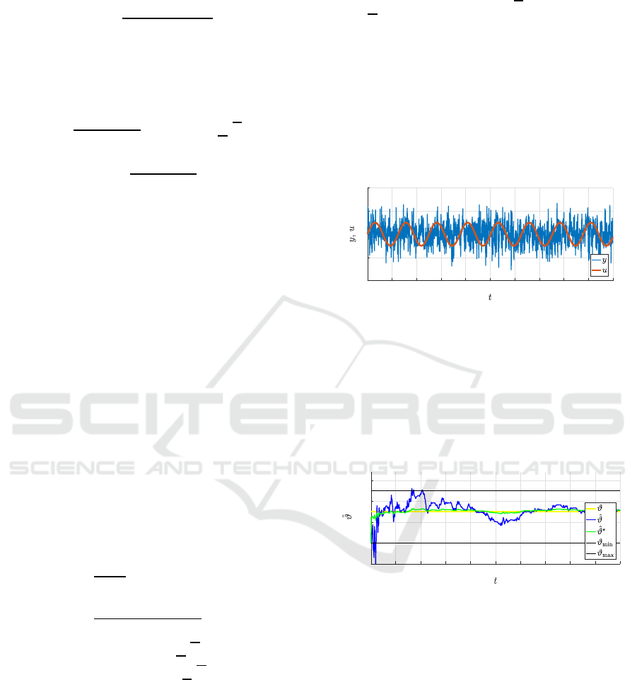
4.1.1 Illustrative Example

Consider a model

y(t) = ϑu(t − 1) + e

(t) (43)

with one parameter

ϑ = 0.15 , (44)

where boundaries, noise and number of steps are

= 0.0 ϑ = 0.25

(t) ∼ N (0,1)

n = 1000

(45)

The control signal was generated according to equa-

tion

u(t) = sin(t/20) . (46)

Behaviour of input u(t) and output y(t) are shown

in Fig. 3. Due to intentionally big variance of the sys-

tem noise, the harmonic component can be hardly rec-

ognized in the output signal.

0 100 200 300 400 500 600 700 800 900 1000

-4

-2

Figure 3: Special case: single parameter model – behaviour

of input and output.

The unbounded parameter was estimated by the

algorithm described in section 2.2. The bounded esti-

mate resulted from algorithm (42). Behaviour of both

unbounded (blue) and bounded (green) parameter es-

timates is depicted in Fig. 4. Value of the true param-

eter is represented by the yellow line and the black

lines show the given boundaries.

100 200 300 400 500 600 700 800 900 1000

-0.1

0.1

0.2

0.3

Figure 4: Special case: single parameter model – behaviour

of unbounded (blue) and bounded (green) parameter esti-

mates.

4.2 General Case

Exact solution for general case cannot be found be-

cause of the absence of a deﬁnite rule how to modify

an off-diagonal element in a general position within

the information matrix. An alternative solution had to

be found.

Let the parameters of the general model (4) be di-

vided into two parts

θ = [θ

, θ

] , (47)

where θ

is a m

-elements parameter vector for which

limitation should be applied and θ

is a m

-elements

Realistic Estimation of Model Parameters

531

vector of parameters without boundaries. It must hold

m = m

+ m

, m

< m, m

≥ 1 . (48)

Process model which uses all the deﬁned parame-

ters can be called the full model

y = θ

′

+ θ

′

+ e , (49)

where z

, z

are parts of the data vector z (2) which

correspond to the parts of parameter vector (47).

Unbounded estimation can be based on the algo-

rithm from 2.2 while the vector Θ (3) was enlarged by

estimates of parameter variances σ

Θ = [ θ,σ

,σ

] . (50)

Note: Calculation of parameter variances accord-

ing to (9) is inﬂuenced by behaviour of the auxiliary

variable κ deﬁned by (10). It might be better to calcu-

late the variances explicitly in a moving window the

length of which enables to tune sensitivity of the algo-

rithm to variance changes.

4.2.1 Basic Algorithm of Bounded Estimation

The basic algorithm can be divided into following

parts:

• Initialization of V and κ similarly to (41)

• One step of the recursion

– Estimation

Θ = [

θ,

] of the full model.

– Application of the limiting function (27a) on

subset of the estimates

⋆

= ℓ

(

θ, a

,θ

) (51)

Vector of estimated parameters

◦

is now com-

posed by the bounded and unbounded estimates

◦

= [

⋆

] . (52)

4.2.2 Enlarged Algorithm

Bounded parameter estimates

⋆

from the basic al-

gorithm can be, for a particular recursion step, tem-

porarily considered known constants. Then, they can

be – together with corresponding data z

– moved to

the left side of model equation. It results in reduced

model

y−

⋆

′

= θ

′

+ e , (53)

the parameters θ

′

of which can be newly estimated

by the common algorithm from 2.2.

Thus, the basic algorithm is enlarged to consist of

parts

• Initialization of V and κ similarly to (41)

• One step of the recursion

– Estimation

Θ = [

θ,

] of the full model.

– Employment of the limiting function (27a) on

subset of the estimates

⋆

= ℓ

(

θ, a

,θ

) (54)

– Moving

⋆

together with data z

to the left side

to create the reduced model (53)

– Estimation of parameters

⋆

of the reduced

model. Vector of estimated parameters

⋆

now composed by the bounded estimated pa-

rameters of the full model and by the modi-

ﬁed estimate of unbounded parameters coming

from the reduced model

⋆

= [

⋆

] . (55)

The enlarged algorithm ensures lesser prediction

error than the basic algorithm. In many real cases is

the prediction error even comparable to the one of the

entirely unbounded estimate. Particular results can be

inﬂuenced by the choice of forgetting factors for esti-

mation of the full and reduced models.

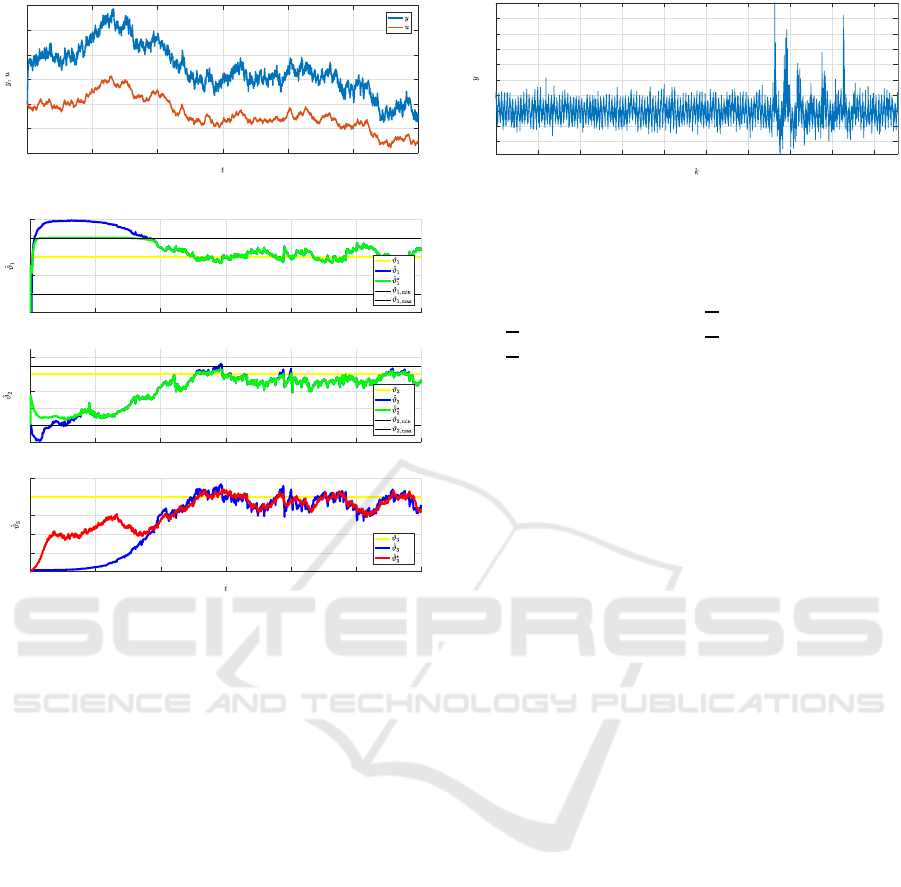
4.2.3 Simulated Example

Consider a process model

y(t) = ϑ

y(t − 1) + ϑ

u(t − 1) + ϑ

+ e

(t) (56)

with parameters

= 0.8 ϑ

= 0.3 ϑ

= 4.0

(57)

and given boundaries, noise and number of samples

= 0.6

= 0.9

= 0.0

= 0.35

(t) ∼ N (0,1)

n = 5000

(58)

The control signal was generated from

u(t) = u(t − 1) + e

(t) , (59)

where e

(t) is a random variable with the uniform dis-

tribution e

(t) ∼ U(−0.5,0.5).

Behaviour of input u(t) and output y(t) is shown

in Fig. 5.

Behaviour of parameter estimates is depicted in

Fig. 6. True parameters are represented by yellow

lines while black lines in the ﬁrst two graphs repre-

sent their given boundaries. Unbounded estimates are

depicted in blue while the bounded ones are green.

The estimate of the single-parameter reduced model

is plotted in red in the lowermost graph.

ICINCO 2017 - 14th International Conference on Informatics in Control, Automation and Robotics

532

0 500 1000 1500 2000 2500 3000

-20

-10

Figure 5: Simulated example – input and output.

500 1000 1500 2000 2500 3000

0.5

0.6

0.7

0.8

0.9

500 1000 1500 2000 2500 3000

-0.1

0.1

0.2

0.3

0.4

0 500 1000 1500 2000 2500 3000

Figure 6: Simulated example – behaviour of unbounded

(blue) and bounded (green) parameter estimates. Estimated

parameter of the reduced model is plotted in red.

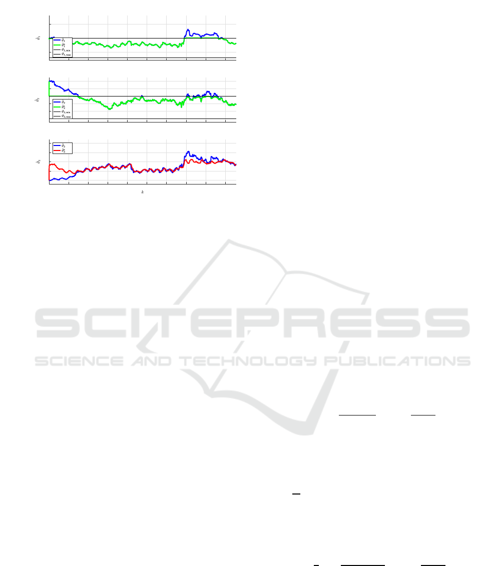
4.2.4 Real Data Example

The example is based on the real data set which was

used in (Ettler and K´arn´y, 2010). System output y is

represented by deviation of the output strip thickness

during the process of cold rolling. Its behaviour is

being approximated by the model

y(k) = ϑ

u(k− 1) + ϑ

v(k− 1) + ϑ

+ e

(k) , (60)

where index k means sample number while the sam-

pling is triggered by the movement of the rolled strip

and ∆k ∼ 0.08 m of the strip length. Control signal u

corresponds to so-called uncompensated rolling gap

of the rolling mill and the measured disturbance v is

represented by the nonlinear function of the rolling

force. The model is based on the gaugemeter princi-

ple, see, e.g. (Ettler and Andr´ysek, 2007) for details.

Fig. 7 shows undesirable variations of measured

output thickness in the interval k ∈ (3300, 4200)

which was caused by dirt inﬂuencing the contact

thickness measurement.

Situation depicted in Fig. 7 caused a temporary

discrepancy between both sides of the model (60)

which may drive unbounded parameter estimates out

of their reasonable ranges.

500 1000 1500 2000 2500 3000 3500 4000 4500

-20

-10

Figure 7: Real data example – the measured output.

Based on the knowledgeof the process, it was pos-

sible to determine boundaries for the ﬁrst two model

parameters:

= −1.0

= −0.02

= −100.0

= 0.00

n = 4700

(61)

Behaviour of parameter estimates is shown in Fig.

8. The second unbounded parameter (in blue)

needs relatively long time k ∈ h1, 700i to reach the

allowed range, which can be explained by a moderate

excitation of the model because selected data come

from the middle of the rolled strip. Concerning the

bounded estimation, the situation is balanced by the

parameter of the reduced model (in red) in the third

graph.

Note: Real on-line identiﬁcation starts with the

beginning of rolling when the system is excited

enough. Here the off-line identiﬁcation starts in the

steady-state to illustrate behaviour of the estimator

under unfavorable conditions.

As a consequence of the measurement error dur-

ing k ∈ (3300, 4200), the blue unbounded estimates

exceeded their limits. The bounded estima-

tor coped with the problem reasonably which is il-

lustrated by the behaviour of the green bounded esti-

mates. Again, the red parameter of the reduced model

deviated from its unbounded version to minimize the

prediction error.

5 CONCLUSIONS

The paper deals with the realistic estimation of model

parameters which takes into account limitation on

model parameters existing in real applications.

In general, limitation of a random variable with

normal distribution N is described by the introduced

heterogenous probability distribution D. Relations

between mean and variance of both distributions can

be adequately approximated by cdf and pdf of the

generalized normal distribution G, respectively. After

Realistic Estimation of Model Parameters

533

500 1000 1500 2000 2500 3000 3500 4000 4500

-0.5

0.5

500 1000 1500 2000 2500 3000 3500 4000 4500

-100

-80

-60

-40

-20

500 1000 1500 2000 2500 3000 3500 4000 4500

100

150

200

Figure 8: Real data example – behaviour of unbounded

(blue) and bounded (green) parameter estimates. The es-

timated parameter of the reduced model is plotted in red.

determination of rules for construction of the ﬁctive G

it was possible to introduce the limiting functions for

the mentioned statistical moments and integrate them

into recursive algorithm of bounded parameter esti-

mation. In addition, parallel estimation of the full and

reduced models enable to minimize the prediction er-

ror in each estimation step.

Behaviour of the estimator was illustrated on

simulated data and then on real data taken from a

cold rolling mill.

REFERENCES

Astr¨om, K. J. and Kumar, P. (2014). Control: A perspective.

Automatica, (50):3–43.

Benavoli, A., Chisci, L., Farina, A., Ortenzi, L., and Zappa,

G. (2006). Hard-constrained vs. soft-constrained pa-

rameter estimation. IEEE Transactions on aerospace

and electronic systems, 42(4):1224 – 1239.

Ettler, P. and Andr´ysek, J. (2007). Mixing models to im-

prove gauge prediction for cold rolling mills. In Pro-

ceedings of the 12th IFAC Symposium on Automation

in Mining, Mineral and Metal Processing, Qu´ebec,

Canada.

Ettler, P. and K´arn´y, M. (2010). Parallel estimation respect-

ing constraints of parametric models of cold rolling. In

Proceedings of the 13th IFAC Symposium on Automa-

tion in Mineral, Mining and Metal Processing (IFAC

MMM 2010), pages 63–68, Cape Town, South Africa.

K´arn´y, M. (1982). Recursive parameter estimation of re-

gression model when the interval of possible values is

given. Kybernetika, 18(2):164–178.

K´arn´y, M., B¨ohm, J., Guy, T., Jirsa, L., Nagy, I., Nedoma,

P., and Tesaˇr, L. (2005). Optimized Bayesian Dynamic

Advising: Theory and Algorithms. Springer, London.

Kopylev, L. (2012). Constrained parameters in applications:

Review of issues and approaches. ISRN Biomathemat-

ics, 2012:Article ID 872956.

Kulhav´y, R. and Zarrop, M. B. (1993). On a general con-

cept of forgetting. International Journal of Control,

58(4):905–924.

Mandelkern, M. (2002). Setting conﬁdence intervals for

bounded parameters. Statistical Science, 17(2):194–

172.

Milanese, M., Norton, J., Piet-Lahanier, H., and (Eds.),

E. W. (1996). Bounding Approaches to System Identi-

ﬁcation. Springer.

Murakami, K. and Seborg, D. E. (2000). Constrained pa-

rameter estimation with applications to blending op-

erations. Journal of Process Control, 10:195–202.

Norton, J. P. (1987). Identiﬁcation and application of

bounded-parameter models. Automatica, 23(4):497–

507.

Peterka, V. (1981). Bayesian Approach to System Identiﬁca-

tion In P. Eykhoff (Ed.) Trends and Progress in System

Identiﬁcation. Pergamon Press, Eindhoven, Nether-

lands.

Toulias, T. L. and Kitsos, C. P. (2014). On the proper-

ties of the generalized normal distribution. Discus-

siones Mathematicae Probability and Statistics, 34(1-

2):3549.

APPENDIX

Generalized Normal Distribution

Symmetric version of the generalized normal distribution

G is deﬁned by 3 parameters: µ

(location), α (scale) and

β (shape).

Pdf of G is given by

(x| µ

,α, β) =

2αΓ(1/β)

exp

(

−



x− µ



)

, (62)

where α > 0, β > 0 and Γ denotes the gamma function

Γ(x) =

∞

x−1

exp(−t)dt . (63)

For β = 2, G coincides with the normal distribution

N (µ

). For β → ∞, G converges pointwise to uniform

density on (µ

− α,µ

+ α).

Cdf of G is given by

(x| µ

,α, β) = (64)

sgn(x− µ

)

Γ(1/β)

1/β,



x− µ



where γ means the lower incomplete gamma function

γ(x,x

) =

x−1

exp(−t)dt . (65)

Remaining properties of G can be found for example in

(Toulias and Kitsos, 2014).

ICINCO 2017 - 14th International Conference on Informatics in Control, Automation and Robotics

534