Accuracy Analysis and Improvement for Cooperative Industrial Robots
M. Wagner
1
, A. Buschhaus
2
, S. Reitelsh
¨
ofer
2
, P. Heß
3
and J. Franke
2
1
Nuremberg Campus of Technology (NCT), Nuremberg Institute of Technology, 90429 Nuremberg, Germany
2
Institute for Factory Automation and Production Systems (FAPS), Friedrich-Alexander-Universit
¨
at
Erlangen-N
¨
urnberg (FAU), 91058 Erlangen, Germany
3
Faculty of Mechanical Engineering and Building Services Engineering, Nuremberg Institute of Technology,
90489 Nuremberg, Germany
Keywords:
Accuracy, Calibration, Industrial Robots, Multi-robot Systems.
Abstract:
The cooperative working of multiple robots on a common task often requires a high geometric accuracy. If
such a system is modeled, many sources of error are present, which can quickly lead to inadequate process
results. In order to avoid this, it is important to carry out a calibration in which deviations are determined.
Subsequently, the model can be adapted to the actual conditions. In the scope of this work a kinematic
calibration method for multi-robot systems is developed and realized with a robot setup consisting of two
industrial robot arms. The accuracy of the robot system is significantly improved by the developed approach,
which has been proven by experimental investigations.
1 INTRODUCTION
The accuracy of industrial robots has been under in-
vestigation for many years. Due to the current devel-
opment of new industrial robot applications the ac-
curacy gets more and more important. For example,
high precision processes, like robot-based medical in-
terventions (Boctor et al., 2004; Baron et al., 2010),
are implemented using industrial robots. In addition,
the number of processes programmed by offline pro-
gramming rises and it is important to ensure a suf-
ficient accuracy for these applications by matching
the virtual model of the robot with the corresponding
real robot. Therefore, many approaches for the im-
provement of the robot accuracy are developed. Since
the changing of the mechanical structure is connected
with a large expenditure, most commonly a calibra-
tion is done. Thus, the robot positioning accuracy is
improved by detecting and compensating the error be-
tween the robot model and the real robot.
Another trend in industrial robotics is the use
of multi-robot systems. Hence, applications can
be improved or developed by a cooperation be-
tween multiple robots. The coordination between
the involved robots may have four different levels
(Wagner et al., 2014). In the first level, no coordi-
nation is done between the robots. Thus, the coor-
dination must be considered in advance by the pro-
grammer. If the robots move independently, but re-
ceive individual signals from each other, this is called
asynchronous coordination. As a result, for exam-
ple, the transfer of workpieces can be coordinated. If
the motions of the robots are linked by simple state-
ments, this is called semi-synchronous coordination.
The common lifting of heavy loads, as presented in
(M
¨
uller et al., 2011) and in (Knepper et al., 2013),
is an example for this kind of coordination. A more
complex coordination of the movements is called syn-
chronous coordination. In this case, for example, a
common base movement is carried out while a robot
is performing a superimposed processing movement,
as shown in (Smits et al., 2008). Another example
presented in (Wagner et al., 2014) is the cooperative
processing by dividing the process movement in a tool
and a workpiece movement.
More complex cooperative processes are often
programmed offline, since the effort would otherwise
be disproportionate. Also for cooperative processes
a maximum match between the model and the real
robot is very important in order to ensure a suffi-
cient relative accuracy between the robots. An ex-
ample for a cooperative process with a requirement
of a high accuracy is the incremental sheet metal
forming by two cooperating industrial robot arms
(Meier et al., 2009). Also for the cooperative process-
ing, presented in (Wagner et al., 2014), a high accu-
racy is necessary. Thus, a new approach for the im-
provement of the accuracy of multi-robot systems is
Wagner, M., Buschhaus, A., Reitelshöfer, S., Heß, P. and Franke, J.
Accuracy Analysis and Improvement for Cooperative Industrial Robots.
DOI: 10.5220/0006396805390546
In Proceedings of the 14th International Conference on Informatics in Control, Automation and Robotics (ICINCO 2017) - Volume 2, pages 539-546
ISBN: Not Available
Copyright © 2017 by SCITEPRESS – Science and Technology Publications, Lda. All rights reserved
539

presented in the scope of this paper.
This paper is structured as follows: Section 2
gives an overview about the current state of the art in
kinematic calibration. Subsequently, the researched
method for the accuracy improvement for cooperative
industrial robots is presented in Section 3. The im-
plementation of the approach with a setup consisting
of two industrial robot arms is explained in Section 4.
The last section concludes the paper.
2 KINEMATIC CALIBRATION
The aim of the kinematic calibration is the minimiza-
tion of the deviation between the current path and the
target path of the robot movement. The kinematic
calibration can be carried out according to two ba-
sic principles (Day, 1996). On the one hand it can be
done by an inline calibration using closed-loop cor-
rection (Buschhaus et al., 2016). Here, the error is
detected and compensated during the processing. On
the other hand the calibration can be performed by an
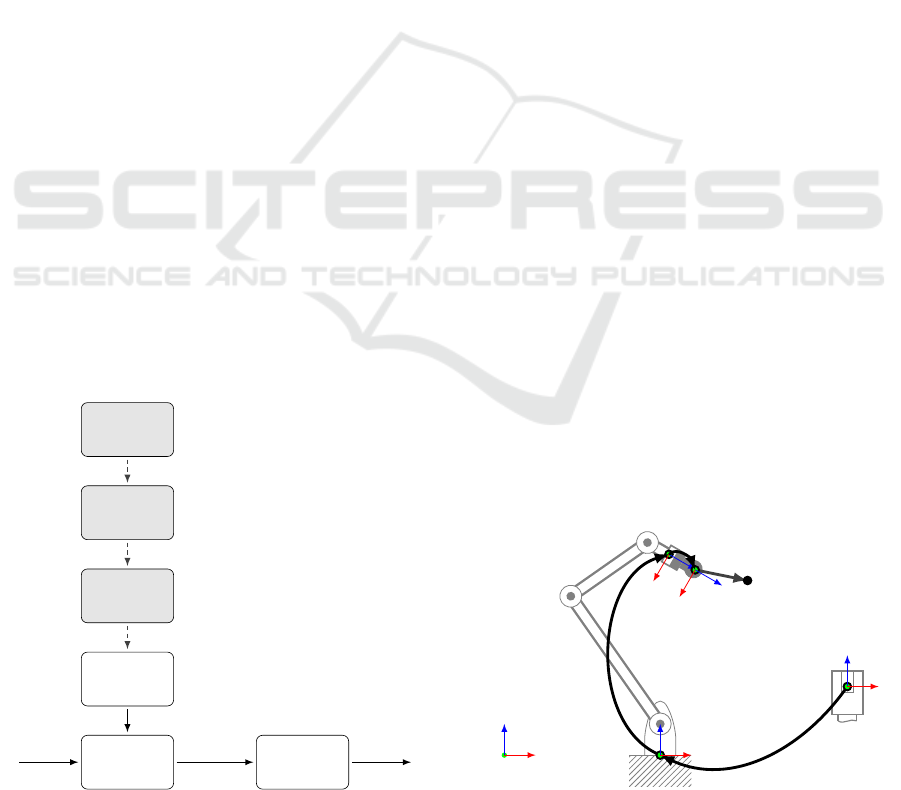
open-loop correction (see Figure 1). In doing so, the
error in the system is recorded once in a measuring
process and the kinematic model is adapted accord-
ingly.
According to (Elatta et al., 2004), the kinematic
calibration consists of four sequential steps. First, the
robot kinematics is modeled. Second, the necessary
measurements are performed. Third, the calibration
parameters are estimated based on the measured data.
Finally, the calculated calibration parameters are used
to adjust the kinematic model and thus to compensate
the error. These four steps are explained in the fol-
lowing subsections.
Inverse
Kinematics
Robot
Model of
Kinematics
Compen-
sation
Identifi-
cation
Measure-
ments
Desired
Pose
Axis
Values
Robot
Pose
Figure 1: Open-loop correction method for industrial
robots.
2.1 Modeling
The considered robot has a base coordinate system
{B} (see Figure 2) which is usually located inside of
the robot base. Thus, the exact position of the base
coordinate system is unknown. The pose of the flange
{F} results from the kinematics of the robot and is de-
scribed by the transformation
B
T
F
. For common ap-
plications the tool center point (TCP) {T } is located
in front of the flange. The equivalent transformation
is denoted by
F
T
T
.
Furthermore, two calibrations have to be per-
formed in advance in order to achieve a sufficient
accuracy. First, the exact base coordinate system
{B} must be determined. Thus, the base transforma-
tion
S
T
B
has to be measured indirectly and calculated
based on geometric relations. Second, the transforma-
tion between the robot flange and the TCP
F
T
T
needs
to be determined. Even if the tool is produced with
high accuracy, there is still a relevant inaccuracy in
its installation to the robot flange. If the base of the
tool is not reachable by a mechanical measuring in-
strument, it has to be determined by a calibration pro-
cedure as well.
2.2 Measurements
During the measurements, the position of the TCP in
the workspace of the robot is recorded. Various mea-
surement methods, e.g. acoustic or visual sensors as
well as coordinate measuring machines, can be used
for this purpose. Most of the approaches use auto-
matic theodolites, also known as laser tracker, due
to their high precision (Alicia and Shirinzadeh, 2005;
Nguyena et al., 2015).
The definition of the measurement positions de-
pends on the respective applications. Thus, in (Alicia
and Shirinzadeh, 2005) 80 positions are used to cover
the range of motions for example. In order to reduce
the number of positions, the optimal measuring posi-
{F}
e
i
{T }
p
S
T
B
{S}
B
T
F
F
T
T
{B}
y
z
x
Figure 2: Coordinate systems at the accuracy analysis for
industrial robots.
ICINCO 2017 - 14th International Conference on Informatics in Control, Automation and Robotics
540

tions can be selected by using a genetic algorithm in
(Aoyagi et al., 2010).
2.3 Identification
Each of the N measured positions p
a
= (x
a
y
a
z
a
)
T
can be compared with the corresponding desired
position p
d
= (x
d
y
d
z
d
)
T
. Thus, an error vector
e = (x
e
y
e
z
e
)
T
can be calculated according to:
e
i
= p
a
i
− p
d
i
, i ∈ {1, 2, . . . , N} (1)
Furthermore, the error ε of a position can be indi-
cated by the distance between the two points by:
ε
i
= ||e
i
|| =
=
q
(x
a
i
− x
d
i
)
2
+ (y
a
i
− y
d
i
)
2
+ (z
a
i
− z
d
i
)
2
,
i ∈ {1, 2, . . . , N}
(2)
2.4 Compensation
In the final step of the kinematic calibration, the kine-
matic model of the robot is adapted according to
the identified errors. The error consists of geomet-
rical and non-geometrical errors (Elatta et al., 2004;
Nguyena et al., 2015). Geometrical errors result from
deviations in the link length or twist errors and can be
determined relatively easy. Thus, e.g. the joint an-
gle error can be estimated by a calibration, as shown
in (Chen et al., 2008) by tracking a laser line in the
robot workspace. Most of the approaches calculate
the geometrical error based on the measurement of
multiple robot positions with an external high preci-
sion measurement unit and a calculation of the devi-
ation based on alorithms like extended Kalman filter-
ing (Nguyena et al., 2015), root mean square (Alicia
and Shirinzadeh, 2005) or non-linear least squares op-
timization (Lightcap et al., 2008; Aoyagi et al., 2010).
Non-geometrical errors, such as gear backlash or join
and link flexibility, are more difficult to determine.
Some approaches use an artificial neural network to
compensate this errors (Nguyena et al., 2015; Aoy-
agi et al., 2010). Other approaches try to model the
non-geometrical errors, e.g. with a class of polynom-
inals (Alicia and Shirinzadeh, 2005) or a Monte Carlo
simulation (Lightcap et al., 2008).
3 APPROACH
For the cooperative processing, the relative accuracy
between the robots is of importance. Thus, it is an-
alyzed by measuring the absolute accuracy for both
robots and by calculating the deviation between both
measurements. Subsequently, the systematic error is
compensated by an adaption of the kinematic model.
According to the previous section, this section is di-
vided into the same four subsections.
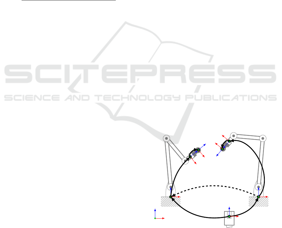
3.1 Modeling
At least two robots are required for cooperative pro-
cessing (see Figure 3). In the following, the terms
workpiece guiding robot and tool guiding robot are
used for the involved robots. However, several robots
can also guide the workpiece or the tool. Each robot
has a transformation from its base to its flange, de-
noted by
B
T
T
F
T
and
B
W
T
F
W
. Furthermore, each robot
has a transformation from its flange to its TCP. This
also applies to the reflector {R} used for examining
the accuracy by a laser tracker. The transformations to
the center of the reflectors are
F
T
T
R
T
and
F
W
T
R
W
. The
transformation between the two robot base frames is
denoted by
B
T
T
B
W
. In addition, the transformations
between the sensor base frame {S} and the two robot
base frames, denoted by
S
T
B
T
and
S
T
B
W
, are relevant.
According to Section 2.1, a base and a tool cal-
ibration must also be carried out in advance for the
cooperative approach. Thus, for each robot a base
transformation, denoted by
S
T
B
T
and
S
T
B
W
, as well
as a reflector transformation, denoted by
F
T
T
R
T
and
F
W
T
R
W
, are determined.
{F
T
}
{R
T
}
{R
W
}
{B
W
}
{F
W
}
S
T
B
T
S
T
B
W
B
T
T
B
W
{S}
B
T
T
F
T
F
T
T
R
T
B
W
T
F
W
F
W
T
R
W
{B
T
}
y
z
x
Figure 3: Coordinate systems at the accuracy analysis for
cooperative processing.
Accuracy Analysis and Improvement for Cooperative Industrial Robots
541

3.2 Measurements
The investigation focuses on the part of the
workspace which is relevant for the coopera-
tive processing—the common workspace. In order to
limit the amount of measurements, measuring points
are equally distributed within the common workspace
by an algorithm (see Figure 4). The algorithm runs
with a constant step size from the bottom to the top of
a box containing the workspace. In order to keep the
robot paths to a minimum, the x-direction is toggled.
Each iterated position is checked for reachability by
inverse kinematics and the position will be added to
the measurement positions, if it is reachable.
The algorithm generates programs for both robots
that enables them to move the reflector to the absolute
set poses of the accuracy analysis path. Due to the
inaccuracies in the system, each robot movement has
a deviation compared to the pre-defined path.
3.3 Identification
Based on the measurement results, the relative de-
viations between the measured positions and the de-
sired positions is calculated via Equation 1 and Equa-
tion 2. However, the relative position between the two
robots is essential for the cooperative process. Thus,
the equations are adapted to the relative deviation be-
tween the two robot poses. The error vector e results
from the difference between the measured tool posi-
1: procedure GENERATE PATHS(S
k
)
2: for z ← z
min
, z
max
do
3: for y ← y
min
, y
max
do
4: if toggle then
5: for x ← x
min
, x
max
do
6: if REACHABLE(x, y, z) then
7: commands → programs
8: end if
9: end for
10: else
11: for x ← x
max
, x
min
do
12: if REACHABLE(x, y, z) then
13: commands → programs
14: end if
15: end for
16: end if
17: toggle ←!toggle
18: end for
19: end for
20: end procedure
Figure 4: Procedure for creating the robot paths with
equally distributed measurement points for the accuracy
analysis for cooperative processing.
tion p
T
and the measured workpiece position p
W
by:
e
i
= p
T
i
− p
W
i
, i ∈ {1, 2, . . . , N} (3)
The absolute error ε at the position results from
the distance between the two measured positions by:
ε
i
= ||e
i
|| =
=
q
(x
T
i
− x
W
i
)
2
+ (y
T
i
− y
W
i
)
2
+ (z
T
i
− z
W
i
)
2
,
i ∈ {1, 2, . . . , N}
(4)
Furthermore, a compensation transformation T
C
can be calculated from all of the deviations by the It-
erative Closest Point (ICP) algorithm (Zhang, 1992).
In the course of this, the transformation is determined
by an interative minimization of the distances be-
tween the point clouds.
3.4 Compensation
The open-loop correction method presented in Sec-
tion 2 is modified in order to adapt the desired pose of
the workpiece guiding robot (see Figure 5). For this
purpose, the base transformation
B
T
T
B
W
is adapted
using the compensation transformation T
C
. The
compensation transformation consists of a translation
t
C
= (x
C
y
C
z
C
)
T
and a rotation r
C
= (α
C
β
C
γ
C
)
T
.
Based on these parameters, the base transformation
between the two robots can be modified by:
B
T
T
0
B
W
=
B
T
T
B
W
· T
C
(5)
Accordingly, a target pose for the workpiece guid-
ing robot
B
W
T
P
can be determined by the target pose
of the tool guiding robot
B
T
T
P
according to the equa-
tion:
B
W
T
P
= (T
C
)
−1
·

B
T
T
B
W

−1
·
B
T
T
P
=
=

B
T
T
0
B
W

−1
·
B
T
T
P
(6)
Compen-
sation
Inverse
Kinematics
Robot
Model of
Kinematics
Identifi-
cation
Measure-
ments
Desired
Pose
Axis
Values
Robot
Pose
Comp.
Pose
Figure 5: Open-loop correction method for the desired pose
of cooperative industrial robots.
ICINCO 2017 - 14th International Conference on Informatics in Control, Automation and Robotics
542

4 IMPLEMENTATION &
RESULTS
The previously described approach is implemented
with a robot setup consisting of two industrial robot
arms. The setup is presented in the next subsection.
Subsequently, the realization of the preliminary cali-
brations is explained. In the last subsection the real-
ization of the measurements and the resulting data is
presented.
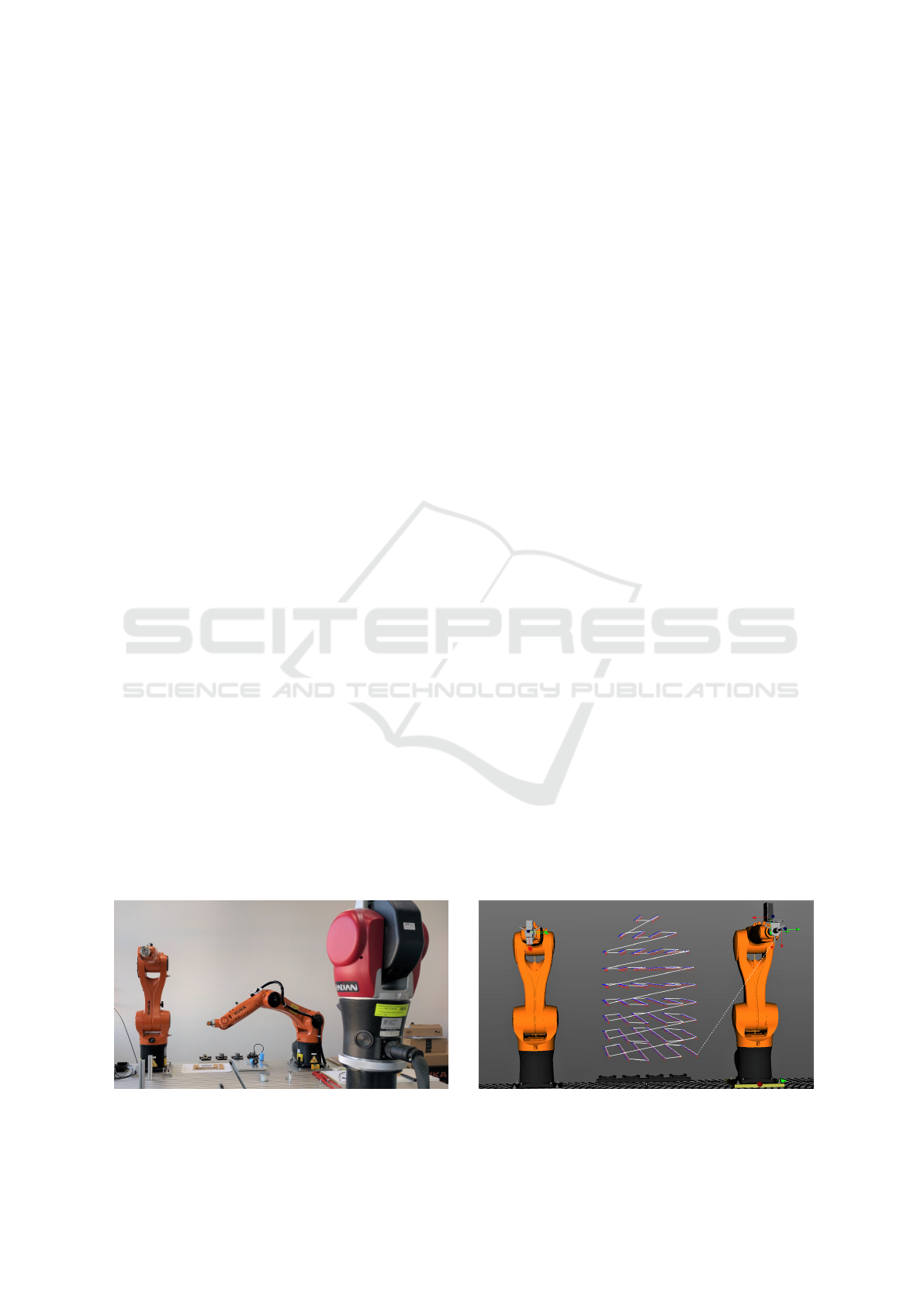
4.1 Setup
The robotic system used for the investigation con-
sists of two KUKA KR 6 R900 sixx industrial robot
arms (see Figure 6). They are mounted next to each
other with a distance of approximately 1325 mm in
y-direction. Each robot arm consists of six axis and a
position repeatability of ±0.03 mm according to man-
ufacturer specifications.
The laser tracker API R-20 Radian is used as an
external measuring device. It is placed in front of the
robots to be able to measure within the entire common
workspace. Each robot has a reflector mounted to its
flange via an adapter plate.
4.2 Calibrations
According to Section 3.1, two calibrations have to
be performed before the measurements. First, the
base coordinate systems of the robots have to be
determined. They are measured by mounting a re-
flector on the rotating part of the robot next to the
first and the second rotational axis. For both axes a
measurement is performed by rotating the axes. This
results in a circular path whose center point lies in the
rotational axis. The actual robot base can be deter-
mined via the intersection of the resulting rotational
axes.
Figure 6: Setup for the accuracy analysis for cooperative
industrial robots.
Furthermore, the transformation between the two
robots base coordinate systems can be determined by:
B
T
T
B
W
=

S
T
B
T

−1
·
S
T
B
W
(7)
The resulting base transformation for the
examined setup consists of a translation of
t
B
= (3.18 − 1319.28 0.17)
T
in mm and a ro-
tation of r
B
= (0.00 0.01 0.26)
T
in degree.
Second, the translation between the flange and
the mounted reflector needs to be determined. Since
the fixing adapter is produced with a very high accu-
racy in radial direction, a low eccentricity is assumed.
Therefore, only the offset in z-direction is estimated
by the calibration. For this purpose, the robot per-
forms a pitch rotation around its flange axis. Thereby,
a circular path of the reflector can be recorded. The
z-offset is equivalent to the radius of the fitting cir-
cle. The resulting values for the considered setup
are z
R
T
= 36.79 mm for the tool guiding robot and
z
R
W
= 36.71 mm for the workpiece guiding robot.
4.3 Measurements & Data
The measurement paths for both robots are gener-
ated according to Section 3.2. The resulting programs
contain movements inside the common workspace of
both robots, which are aligned on a uniformly dis-
tributed grid (see Figure 7). After each movement
command the program contains a wait-command to
ensure a measurement at the desired position. The
generated path consist of a total of 472 measurement
positions.
Based on the measurement results, the relative de-
viations between the matching positions can be calcu-
lated by Equation 3 and Equation 4. Figure 8(a)-8(c)
show the resulting deviations divided in x-, y- and
z-direction. The magnitude of the deviation is directly
proportional to the length of the line and the lines are
colored according to a heatmap, which is shown in
Figure 8(d).
Figure 7: Generated robot path for the tool guiding robot
for the accuracy analysis.
Accuracy Analysis and Improvement for Cooperative Industrial Robots
543

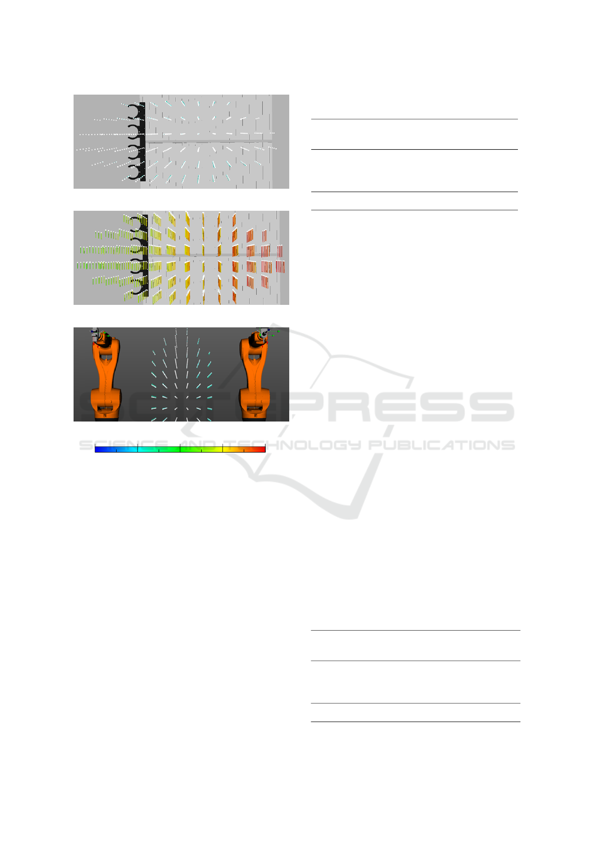
(a) Deviation in x-direction.
(b) Deviation in y-direction.
(c) Deviation in z-direction.
0 2 4
6
8
x
e
, y
e
, z
e
in mm
(d) Heatmap.
Figure 8: Accuracy maps with scaled deviations colored by
a heat map depending on the absolute value.
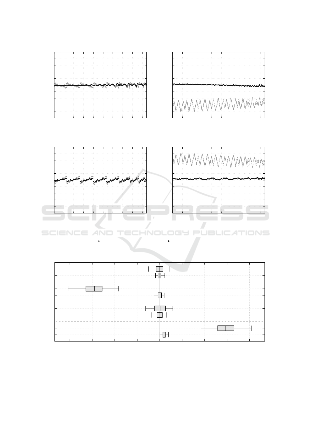
Furthermore, the deviation values are summarized
in diagrams (see Figure 9) in order to get a better
overview. Here, all measurement points are listed in
sequence. Each axial direction (x
e
, y
e
, z
e
) is presented
in a separate diagram as well as the absolute error ε.
The distribution of the deviations before the com-
pensation is presented in Table 1.
The deviation in x- and z-direction varies in
the range between about -1.0 mm and 1.0 mm.
A comparatively large negative deviation in the
y-direction is obvious, which presumably is due to
the oppositeness of the two robots in this direction.
This deviation is decisive for the absolute error with
a maximum of more than 8.0 mm. The standard
deviations before the compensation are in the range
of 0.40 mm to 0.96 mm.
Table 1: Distribution of relative positional deviations for the
cooperative robot system.
¯
e min(e) max(e) σ(e)
(mm) (mm) (mm) (mm)
x
e
-0.0262 -1.0007 0.9037 0.4044
y
e
-5.8465 -8.1463 -3.6525 0.9559
z
e
0.0087 -1.2508 1.1629 0.6119
ε 5.8925 3.6713 8.1544 0.9547
According to Section 3.4, a compensation is per-
formed. The resulting compensation transformation
for the considered setup consists of a translation of
t
C
= (−1.81 6.96 1.41)
T
in mm and a rotation of
r
C
= (0.16 0.00 0.12)
T
in degree. The deviations
after the compensation are also shown in the diagrams
(see Figure 9). Table 2 shows the distribution of the
deviations after the compensation. The mean error
vector tends to zero and all deviations are less than
0.8 mm. The standard deviations after the compensa-
tion are between 0.14 mm and 0.31 mm. In order to
provide better comparability, the data is displayed in
a box-and-whisker diagram (see Figure 10).
5 CONCLUSIONS
In the scope of this paper an approach for the im-
provement of the accuracy for cooperative industrial
robots is developed. Thus, the robots are examined by
means of a high-precision external measuring device.
On the one hand, the approach includes the creation
of robot programs for the measurement. On the other
hand, the estimation of an error compensation is pre-
sented. The approach is implemented with a robot
system with two industrial robot arms for validation.
The comparison of the deviations before and after the
compensation shows a significant reduction of about
90 %. In addition, the variation is significantly re-
duced in comparison to the deviations without com-
pensation.
Table 2: Distribution of relative positional deviations for the
cooperative robot system after the compensation.
¯
e
0
min(e
0
) max(e
0
) σ(e
0
)
(mm) (mm) (mm) (mm)
x
0
e
-0.0001 -0.3687 0.6136 0.1889
y
0
e
0.0001 -0.5031 0.4041 0.2088
z
0
e
0.0000 -0.7086 0.6213 0.3077
ε
0
0.3905 0.0223 0.7938 0.1456
ICINCO 2017 - 14th International Conference on Informatics in Control, Automation and Robotics
544

-10
-8
-6
-4
-2
0
2
4
6
8
10
0 50 100 150 200 250 300 350 400 450
x
e
in mm
Point number
(a) Error in x-direction.
-10
-8
-6
-4
-2
0
2
4
6
8
10
0 50 100 150 200 250 300 350 400 450
y
e
in mm
Point number
(b) Error in y-direction.
-10
-8
-6
-4
-2
0
2
4
6
8
10
0 50 100 150 200 250 300 350 400 450
z
e
in mm
Point number
(c) Error in z-direction.
-10
-8
-6
-4
-2
0
2
4
6
8
10
0 50 100 150 200 250 300 350 400 450
ε in mm
Point number
(d) Absolute error.
Before compensation After compensation
Figure 9: Deviations at the different measurement positions.
−8
−6
−4 −2 0 2 4
6
8
ε
ε
0
z
e
z
0
e
y
e
y
0
e
x
e
x
0
e
Deviation in mm
Figure 10: Box-and-whisker diagram of relative positional deviations for the cooperative robot system.
Accuracy Analysis and Improvement for Cooperative Industrial Robots
545

REFERENCES
Alicia, G. and Shirinzadeh, B. (2005). A systematic tech-
nique to estimate positioning errors for robot accuracy
improvement using laser interferometry based sens-
ing. In Mechanism and Machine Theory, volume 40,
pages 879–906. Elsevier.
Aoyagi, S., Kohama, A., Nakata, Y., Hayano, Y., and
Suzuki, M. (2010). Improvement of robot accuracy
by calibrating kinematic model using a laser track-
ing system-compensation of non-geometric errors us-
ing neural networks and selection of optimal measur-
ing points using genetic algorithm. In Proceedings of
the IEEE/RSJ International Conference on Intelligent
Robots and Systems (IROS 2010), pages 5660–5665.
IEEE.
Baron, S., Eilers, H., Munske, B., Toennies, J. L., Balachan-
dran, R., Labadie, R. F., Ortmaier, T., and III, R. J. W.
(2010). Percutaneous inner-ear access via an image-
guided industrial robot system. In Proceedings of the
Institution of Mechanical Engineers, Part H: Journal
of Engineering in Medicine, volume 224, pages 633–
649. SAGE.
Boctor, E. M., Fischer, G., Choti, M. A., Fichtinger, G., and
Taylor, R. H. (2004). A dual-armed robotic system for
intraoperative ultrasound guided hepatic ablative ther-
apy: a prospective study. In Proceedings of the IEEE
International Conference on Robotics and Automation
(ICRA 2004), volume 3, pages 2517–2522. IEEE.
Buschhaus, A., Gr
¨
unsteudel, H., and Franke, J. (2016).
Geometry-based 6d-pose visual servoing system en-
abling accuracy improvements of industrial robots.
In Proceedings of the International Conference on
Advanced Mechatronic Systems (ICAMechS 2016),
pages 195–200. IEEE.
Chen, H., Fuhlbrigge, T., Choi, S., Wang, J., and Li, X.
(2008). Practical industrial robot zero offset cali-
bration. In Proceedings of the IEEE International
Conference on Automation Science and Engineering
(CASE 2008), pages 516–521. IEEE.
Day, C. P. (1996). Robot accuracy issues and methods of
improvement. In Progress in Robotics and Intelligent
Systems, volume 2, pages 90–108. Intellect Books.
Elatta, A., Gen, L., Zhi, F., Daoyuan, Y., and Fei, L. (2004).
An overview of robot calibration. In Information
Technology Journal, volume 3, pages 74–78. Asian
Network for Scientific Information.
Knepper, R. A., Layton, T., Romanishin, J., and Rus, D.
(2013). Ikeabot: An autonomous multi-robot coordi-
nated furniture assembly system. In Proceedings of
the IEEE International Conference on Robotics and
Automation (ICRA 2013), pages 855–862. IEEE.
Lightcap, C., Hamner, S., Schmitz, T., and Banks, S.
(2008). Improved positioning accuracy of the pa10-
6ce robot with geometric and flexibility calibration.
In IEEE Transactions on Robotics, volume 24, pages
452–456. IEEE.
Meier, H., Buff, B., Laurischkat, R., and Smukala, V.
(2009). Increasing the part accuracy in dieless robot-
based incremental sheet metal forming. In CIRP An-
nals - Manufacturing Technology, pages 233–238. El-
sevier.
M
¨
uller, R., Esser, M., and Janssen, M. (2011). Integrative
path planning and motion control for handling large
components. In Proceedings of the 4th International
Conference on Intelligent Robotics and Applications
(ICIRA 2011), pages 93–101. Springer-Verlag, Berlin,
Germany.
Nguyena, H.-N., Zhoua, J., and Kang, H.-J. (2015). A cali-
bration method for enhancing robot accuracy through
integration of an extended kalman filter algorithm and
an artificial neural network. In Neurocomputing, vol-
ume 151, pages 996–1005. Elsevier.
Smits, R., Laet, T. D., Claes, K., Bruyninckx, H., and Schut-
ter, J. (2008). itasc: a tool for multi-sensor integration
in robot manipulation. In Proceedings of the IEEE
International Conference on Multisensor Fusion and
Integration for Intelligent Systems, pages 426–433.
IEEE.
Wagner, M., Heß, P., and Reitelsh
¨
ofer, S. (2014). Auto-
mated programming of cooperating industrial robots.
In Proceedings for the joint conference of 45st Inter-
national Symposium on Robotics (ISR 2014) und 8th
German Conference on Robotics (ROBOTIK 2014),
pages 129–136. VDE-Verlag, Berlin, Germany.
Zhang, Z. (1992). Iterative point matching for registration
of free-form curves. In Technical Report RR-1658.
INRIA Sophia Antipolis, Valbonne Cedex, France.
ICINCO 2017 - 14th International Conference on Informatics in Control, Automation and Robotics
546