
Optimal Scheduling of an on-Demand Fixture Manufacturing Cell for
Mass Customisation Production Systems
Model Formulation, Presentation and Validation
Enrico Naidoo, Jared Padayachee and Glen Bright
Mechatronics and Robotics Research Group, Discipline of Mechanical Engineering, University of KwaZulu-Natal,
King George V Ave, Durban, South Africa
Keywords: Mass Customisation, Reconfigurable Fixtures, Group Technology, Optimisation Model, Mixed Integer
Linear Programming.
Abstract: A focal point of mass customisation production systems (a significant aspect of the fourth industrial
revolution) is the implementation of reconfigurable jigs and fixtures. Traditional methods for the treatment
of conventional fixtures are inadequate for those of the reconfigurable type. This paper describes the
implementation of an on-demand fixture manufacturing cell that would reside in a mass customisation
production system. The focus, in particular, is on the behaviour and optimisation of this cell in relation to
the production system. To achieve this, a multi-stage optimisation procedure was developed that involves
cluster analysis and a mixed inter linear programming (MILP) model to minimise total idle time (and thus
makespan) in the system.
1 INTRODUCTION
The onset of Industry 4.0 has led to an increased
research interest in mass customisation production
systems (Yao and Lin, 2016). A primary focus for
the successful implementation of such production
systems is the topic of reconfigurable jigs and
fixtures (Smith et al., 2013). Customised products
are unique and this has to be accounted for by
employing jigs and fixtures that can accommodate
constantly varying geometries. Reconfigurable jigs
and fixtures are workholding devices that can be
adapted to suit the specifications of each customised
product (Bi and Zhang, 2001). As such, the
scheduling of such a production system has to
consider the reconfigurable fixture as an active
influence on the workflow, and not as a constant
resource.
An on-demand fixture manufacturing cell that
serves a mass customisation production system was
developed as part of this research. This paper
presents an optimisation procedure that schedules
activities within the fixture manufacturing cell in
tandem with a part processing cell. This was
developed as a three-stage process, the last of which
is the primary focus of this paper. The first two
stages involve cluster analysis to optimally assign
parts to fixtures. The third stage utilises a mixed
integer linear programming (MILP) model that
minimises the total idle time in the system caused by
a lack of synchronisation between the two cells.
2 LITERATURE REVIEW
2.1 Fixtures
Fixtures are used to physically locate, hold and
support parts during a manufacturing process. Mass
customisation manufacturing requires fixtures that
can hold parts of varying geometry, and be able to
rapidly and cost effectively change configurations
according to these variations. Reconfigurable
fixtures are a low cost solution to this problem.
Recent advancements include pin-array fixtures and
phase-change materials. The most widely used
reconfigurable fixtures, however, are modular
fixtures. These consist of a constant fixture base
upon which different modules can be attached to
hold various parts (Bi and Zhang, 2001). An
example of such a fixture is the Blüco-Technik®
dowel fixture shown in Figure 1.
Naidoo, E., Padayachee, J. and Bright, G.
Optimal Scheduling of an on-Demand Fixture Manufacturing Cell for Mass Customisation Production Systems - Model Formulation, Presentation and Validation.
DOI: 10.5220/0006396900170024
In Proceedings of the 14th International Conference on Informatics in Control, Automation and Robotics (ICINCO 2017) - Volume 1, pages 17-24
ISBN: 978-989-758-263-9
Copyright © 2017 by SCITEPRESS – Science and Technology Publications, Lda. All rights reserved
17
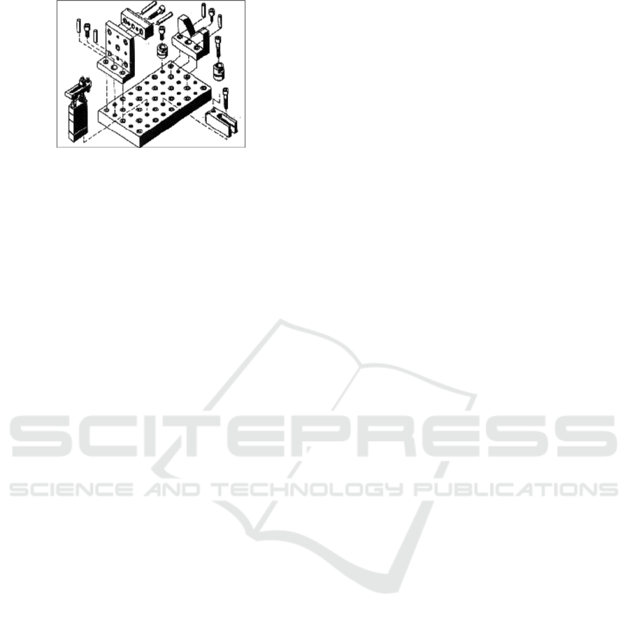
Figure 1: Blüco-Technik® dowel fixture (Bi and Zhang,
2001).
2.2 Group Technology
Mass customisation production systems aim to blend
the advantages of both job shops (high variability
but low volume) and dedicated manufacturing lines
(high volume but low variability) while minimising
their disadvantages (Fogliatto et al., 2012). Group
Technology can play a major role in achieving this.
Group Technology involves clustering similar parts
into part families, which increases the efficiency of
processing since the part family is then
manufactured in a specialised cell. Group
Technology has given rise to the cellular
manufacturing paradigm. Modular fixtures can be
effectively employed in cellular manufacturing
systems, since the fixtures can be specialised for the
part family associated with that cell. The fixtures are
customised according to variations within the part
family by adding and removing various modules
(Groover, 2001).
The modular concept is applied in this research
for implementing an on-demand fixture
manufacturing cell. The fixtures and unfinished parts
are handled separately until the two are assembled at
the point where the part requires the fixture for it to
be machined. The cellular manufacturing method is
used so that modifications can be made to the same
fixture base via fixture reconfigurations to serve
numerous variations of the part type it is associated
with.
2.3 Scheduling and Optimisation
A literary study of scheduling and optimisation
models that considered fixtures as part of the system
was conducted. This involved the typical job shop
scheduling problem and numerous modifications
thereof.
Thörnblad et al., (2013) conducted a study on a
multi-task cell at GKN® Aerospace Engine Systems
in Sweden. The problem was described as a flexible
job shop scheduling problem. A time-indexed
formulation was used. The objective was to
minimise the weighted tardiness, where the
weighting increased as tardiness increased. The task
was to assign a particular fixture to a job, and to
limit the number of fixtures of each type.
A genetic algorithm was used by Wong et al.,
(2009) to solve a resource-constrained assembly job
shop scheduling problem with lot streaming. The
objective was to minimise total lateness cost.
Resource constraints were used to place limits on the
tools and fixtures used in the system, which were
recyclable.
Yu et al., (2012) conducted a study on a
reconfigurable manufacturing system with multiple
process plans and limited pallets/fixtures. The
problem was solved using a priority rule based
scheduling approach, which compromised on
optimality but improved ease of implementation.
This simpler approach allowed the authors to
consider multiple objectives: minimising makespan,
minimising mean flow time, and minimising mean
tardiness. The problem was constrained to only
release jobs once the relevant pallet/fixture was
available.
Literature has revealed that fixture utilisation in a
production system was mostly limited to placing a
constraint on the availability of fixtures as a
resource. There was no research found that dealt
with a system that could manufacture and
reconfigure fixtures on-demand according to the
manufacturing process demands.
3 PROBLEM STATEMENT
3.1 Problem Description
The model presented in this paper describes a
production system where two manufacturing cells
exist to serve fixture reconfigurations and processing
of parts, respectively. This represents a microcosm
of a mass customisation production system that
utilises cellular manufacturing principles to address
the synchronicity required between reconfigurable
fixtures and the customised parts that they serve.
Pre-processed parts are to be processed in the part
processing cell; the fixture configuration required to
hold each of these parts is reconfigured on a fixture
base in the fixture manufacturing cell and delivered
to the part processing cell; each pre-processed part is
then mounted to the fixture base configured for it (its
fixture) so that it can be processed – this is a
fixture-part mapping; the post-processed part is then
ICINCO 2017 - 14th International Conference on Informatics in Control, Automation and Robotics
18
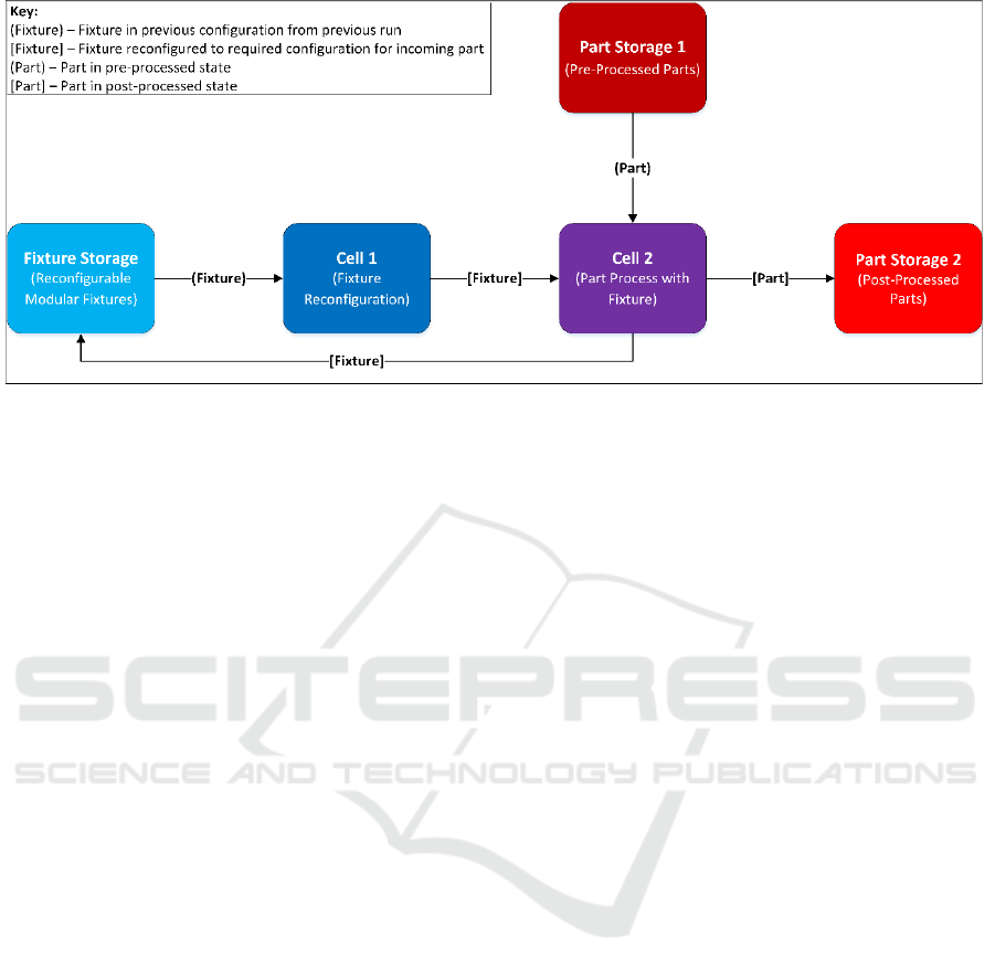
Figure 2: Workflow through the production system being considered.
removed from the fixture and released, while the
fixture returns to the fixture storage system for it to
be reconfigured for another part thereafter. The
workflow through the production system is
described in Figure 2.
The fixtures considered for this problem are of
the reconfigurable modular type. The fixture base
consists of an array of drilled holes. It is
configurable with dowel pins as modules. The
specifications are as follows:
Array pattern: 8x8 holes (64 holes total) per
fixture base;
Pin range: 4-16 pins per fixture configuration.
The problem requires that parts be optimally
assigned to fixture bases such that the interchange
time between fixture configurations per fixture base,
i.e. fixture reconfiguration times, are minimised. The
problem also requires that fixtures be reconfigured
and parts with fixtures be processed synchronously.
These operations must be optimally scheduled such
that the total idle time in the production system is
minimised (thus minimising makespan). The MILP
model presented in this paper focuses on this
problem.
Total idle time was chosen to be the objective
function of the model. This is because delays in the
system would result from the idle time caused by
one cell (either Cell 1 or Cell 2) being occupied after
the other cell has completed its operation, thus
halting workflow in the system. As such, emphasis
has to be placed on ensuring that the operation times
for Cell 1 and Cell 2, for every fixture and part
combination, are as close to each other as possible
for every operation.
3.2 Problem Formulation
The optimisation model presented in this paper is the
final stage of a three-stage model. The three-stage
model aims to solve the problems presented in
Section 3.1 by separating the problem into three
different stages. These are as follows:
1. Clustering Stage - clusters similar parts to be
assigned to the same fixture base by minimising
the dissimilarity measure between the fixture
configurations for those parts.
2. Intracluster Sequencing Stage - sequences the
clustered parts for each fixture base to be ordered
such that the dissimilarities (and the
reconfiguration times, by implication) between
the fixture configurations on that fixture base are
minimised.
3. Final Sequencing Stage - minimises the idle time
in the system by scheduling pairs of fixture-part
mappings that yield a minimised time difference
between their fixture reconfiguration operation
(in Cell 1) and part processing operation (in Cell
2) for every time period.
The model presented in this paper isolates the third
stage only. The first two stages will be briefly
discussed.
The Clustering Stage computes a dissimilarity
measure (an adaptation of the Sokal and Michener
similarity measure (Choi et al., 2010)) for fixture
configurations required for n number parts to be
processed (set P). A comparative matrix is formed
from these values. The measure is non-Euclidean, so
multi-dimensional scaling is used to scale the
comparative distances to a two-dimensional plane,
where k-means clustering is used to cluster the parts
to m number of fixtures (set Q). A fail-safe heuristic
Optimal Scheduling of an on-Demand Fixture Manufacturing Cell for Mass Customisation Production Systems - Model Formulation,
Presentation and Validation
19

is included to ensure that cluster sizes do not force
infeasible solutions. These clusters form the ordered
set I.
The Intracluster Sequencing Stage uses
hierarchical clustering with single linkage to
determine the optimal order of the elements within
each of these clusters. Treating the dissimilarity
measure as a distance, this order ensures that the
shortest distance is traversed for each cluster. This
should ensure that total reconfiguration time for each
fixture base is minimised. The output of this stage is
j
∈
i for each unordered set i
∈
I.
The Final Sequencing Stage can be isolated by
artificially creating the outputs of the first two
stages. This has no influence on demonstrating the
effectiveness of the third stage. This stage only
requires the input of the elements that comprise of
the sets i
∈
I, i.e. n number of parts in m number of
fixtures, distributed feasibly (with 0 representing
empty slots when n is not a multiple of m).
3.3 The Model
The problem is modelled as a mixed integer linear
programming (MILP) problem and solved with a
branch and bound algorithm. The notation for the
entire problem is presented below.
3.3.1 Notation
p; pϵP, P= {1,…,n}
P is the set of parts to be processed;
p is an index of the ordered set P.
q; qϵQ, Q = {1,…,m}
Q is the set of fixtures available; q
is an index of the ordered set Q.
i; iϵI, I={1,…,m}
I is the set of i, i.e. a set of sets that
holds all p-q mappings between sets
P and Q ; i is an index of the
ordered set I.
î; îϵI, I={1,…,m}
î is an alternate index of the ordered
set I.
j; jϵi, i={1,…,|i|}
i is the unordered set of p-q
mappings corresponding
specifically to fixture q, j is an
index of the set i; j denotes a part p
that is mapped to the fixture q.
ĵ; ĵ ϵi, i={1,…,|i|}
ĵ is an alternate index of the
unordered set i.
k; kϵK, K={1,…,n+1}
K is the set of time periods in which
parts or fixtures are processed or
reconfigured, respectively; k is an
index of the ordered set K.
ǩ; ǩϵK, K={1,…,n+1}
ǩ is an alternate index of the ordered
set K.
T
ij
Part processing time; time for part p
corresponding to fixture-part
mapping j
∈
i to be processed; T
ij
is a
parameter.
R
îĵ
Fixture reconfiguration time; time
for fixture î to be reconfigured to
fixture configuration corresponding
to ĵ
∈
î from fixture configuration
corresponding to (ĵ-1)
∈
î
(implicitly), i.e. subsequent
reconfiguration for fixture î; R
îĵ
is a
parameter.
X
ijk
A binary decision variable; X
ijk
= 1
if fixture i is reconfigured for the
fixture-part mapping j
∈
i in time
period k, X
ijk
= 0 otherwise.
ω
iîjĵkǩ
A decision variable; ω
iîjĵkǩ
= 1 if
fixture-part mapping j
∈
i that was
reconfigured in time period k is
processed in time period ǩ=k+1
whilst fixture-part mapping ĵ
∈
î is
synchronously being reconfigured
in time period ǩ, ω
iîjĵkǩ
= 0
otherwise.
φ
iîjĵkǩ
A decision variable; φ
iîjĵkǩ
is the
absolute time difference between
part processing time T
ij
for fixture-
part mapping j
∈
i reconfigured in
time period k, and fixture
reconfiguration time R
îĵ
for fixture-
part mapping ĵ
∈
î reconfigured in
time period ǩ=k+1, i.e. the idle time
for every time period where two
operations are synchronous.
3.3.2 Assumptions
The assumptions used to describe and simplify the
production system for this model are as follows:
Fixture reconfiguration times are known.
There are fewer fixture bases than parts; |Q|<|P|.
The required number of fixtures are already
manufactured and stored, so that only
reconfigurations are now necessary.
Transportation time between fixture
manufacturing cell and part processing cell is
negligible.
Once a part or fixture is assigned to a period k, it
is processed or reconfigured, respectively,
without interruption.
Flow is synchronised between Cell 1 and Cell 2;
a job does not exit Cell 1 until Cell 2 is available,
Cell 1 does not start a new job until the previous
job has exited the cell.
Cell 1 and Cell 2 have a just-in-time workflow
policy (i.e. unit workflow).
The fixture reconfigured in Cell 1 in time period
k is used to process the part assigned to it in
Cell 2 in the next time period ǩ=k+1.
ICINCO 2017 - 14th International Conference on Informatics in Control, Automation and Robotics
20

Figure 3: Example of how the final φ
iîjĵkǩ
decision variables are generated, based on the flow and synchronisation of fixture
reconfiguration operation and part processing operation in either cell.
3.3.3 Mathematical Model
Min
îĵǩ
|
î
|
ĵ
|
|
î
∀
ǩ
1
î
ĵǩ
î
ĵ
∗
î
ĵǩ
∀,∀
î
,∀
∈,∀
ĵ
∈
î
,∀,
∀
ǩ
1
(1)
î
ĵ
ǩ
î
ĵ
∗
î
ĵ
ǩ
0
(1a)
î
ĵ
ǩ
î
ĵ
∗
î
ĵ
ǩ
0
(1b)
î
ĵǩ
∗
î
ĵǩ
∀,∀
î
,∀
∈,∀
ĵ
∈
î
,∀,
∀
ǩ
1
(2)
î
ĵǩ
î
ĵǩ
1
(2a)
î
ĵǩ
0
(2b)
î
ĵǩ
î
ĵǩ
0
(2c)
îĵǩ
|
î
|
ĵ
|
|
î
1
∀
ǩ
1
(3)
ĵǩ
1
∀;∀
∈;∀
ĵ
∈
∈;∀;∀
ǩ
(4)
1
|
|
∀
(5)
1
∀,
∈
(6)
∈
0,1
∀,∀
∈,∀
(7)
î
ĵǩ
0
∀,∀
î
,∀
∈,∀
ĵ
∈
î
,∀,
∀
ǩ
1
(8)
î
ĵǩ
0
∀,∀
î
,∀
∈,∀
ĵ
∈
î
,∀,
∀
ǩ
1
(9)
3.3.4 Model Description
The objective function aims to optimally match the
part processing time for fixture-part mapping j
∈
i and
fixture reconfiguration time for another fixture-part
mapping ĵ
∈
î such that the difference between them
is minimised for time period ǩ=k+1 (which
determines the fixture-part mapping j
∈
i to be
scheduled for fixture reconfiguration in time period
k). This minimises the idle time for either cell for
every time period k.
Constraint (1) calculates the absolute difference
between the part processing time related to
fixture-part mapping j
∈
i in Cell 2 and the fixture
reconfiguration time related to fixture-part mapping
ĵ
∈
î in Cell 1 for time period ǩ=k+1 for every ω
iîjĵkǩ
.
As this constraint is non-linear, Constraints (1a) and
(1b) are used instead of (1) to linearise the absolute
value.
Constraint (2) ensures that the idle times
calculated in Constraints (1a) and (1b) are valid.
This is determined by ensuring that the binary
decision variables related to fixture-part mappings
j
∈
i and ĵ
∈
î for time periods k and ǩ=k+1,
Optimal Scheduling of an on-Demand Fixture Manufacturing Cell for Mass Customisation Production Systems - Model Formulation,
Presentation and Validation
21
respectively (i.e. X
ijk
and X
îĵǩ
), must both be active
(equal to 1) for ω
iîjĵkǩ
>0. As this constraint is
quadratic, Constraints (2a) to (2c) are used instead of
(2) to linearise the non-linearity of (2).
Constraint (3) ensures that the number of ω
iîjĵkǩ
>0
corresponds to the number of time periods in which
Cell 1 and Cell 2 perform operations synchronously,
i.e. one less than the total number of jobs (n-1) since
the first time period hosts an operation in Cell 1 only
(the first fixture reconfiguration).
Constraint (4) imposes the intracluster order on
the final sequence by ensuring that two fixture-part
mappings for the same fixture (j
∈
i and ĵ
∈
i) must
appear in time periods relative to each other that
correspond to the intracluster order (ǩ>k).
Constraint (5) ensures that there is only one
fixture-part mapping j
∈
i assigned to each time
period k. Constraint (6) ensures that each fixture-part
mapping j
∈
i is assigned to a time period k only once
in the schedule.
Constraint (7) is a bound stating that X
ijk
is a
binary variable. Constraints (8) and (9) are bounds
restricting φ
iîjĵkǩ
and ω
iîjĵkǩ
, respectively, to be
non-negative. This ensures that the linearising
constraints for these decisions variables perform
their desired function.
These constraints and bounds limit the problem
search space to remain within the behavioural
boundaries associated with the production system
described in Section 3.1 and the assumptions
presented in Section 3.3.2.
Figure 3 shows an example to demonstrate how
the binary decision variable associated with a given
fixture-part mapping takes on the form of both X
ijk
when in Cell 2 and X
îĵǩ
when in Cell 1. Please note
that the time period index in this figure only
describes the time period value assigned to the
binary decision variable for that absolute time period
- based on the indices of the binary decision variable
(ijk or îĵǩ) for either cell. This is because for
fixture-part mapping 1
∈
1 to be assigned to time
period 1, the operation time in Cell 2 (T
ij
) has to be
considered alongside that for 1
∈
2 (R
îĵ
) when both are
synchronously operated on in time period 2. This
process produces the final decision variable φ
iîjĵkǩ
,
from which the workflow can be easily interpreted
from the indices, as shown in Figure 3.
3.4 Results
The model was solved using the MILP solver
integrated into MATLAB® 2016a. The solver used a
branch and bound algorithm to solve the problems
presented to it.
Problems with a fixture range of 2-4 fixtures and
a part range of 4-16 parts were formulated. The
operation time values were randomised integers
within a range of 15-45 seconds for fixture
reconfiguration operations (R
ij
) and 30-90 seconds
for part processing operations (T
ij
).
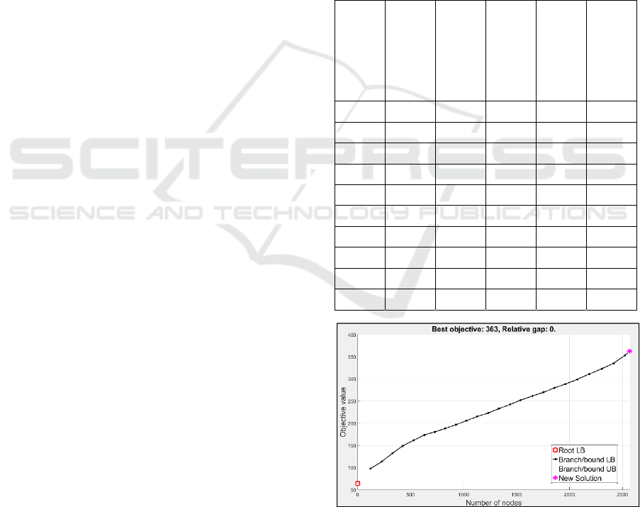
These problems and their solution results are
presented in Table 1. The problems were solved to
optimality. This is shown by the graphs of
convergence for the branch and bound algorithm
(Figure 4 to Figure 6 for a selection of the problems
presented in Table 1).
The test was executed on an Intel® Xeon® CPU
E3-1270 v3 at 3.50 GHz with 16 GB RAM on a
64-bit operating system.
Table 1: Sample problems and results.
Number of
Fixtures
Number of Parts
Number of
Variables
Variable Creation
Time (s)
Solution Time (s)
Convergence
2 4 64 0.044 0.719 Yes
2 6 216 0.111 0.611 Yes
2 8 512 0.424 1.027 Yes
2 10 1000 1.474 5.551 Yes
2 12 1728 4.305 49.12 Yes
3 6 276 0.142 0.752 Yes
3 9 945 1.156 8.583 Yes
3 12 2256 6.510 842.6 Yes
4 8 736 0.762 4.243 Yes
4 12 2520 7.407 6394 Yes
Figure 4: Convergence of 2 fixture/12 part problem.
ICINCO 2017 - 14th International Conference on Informatics in Control, Automation and Robotics
22
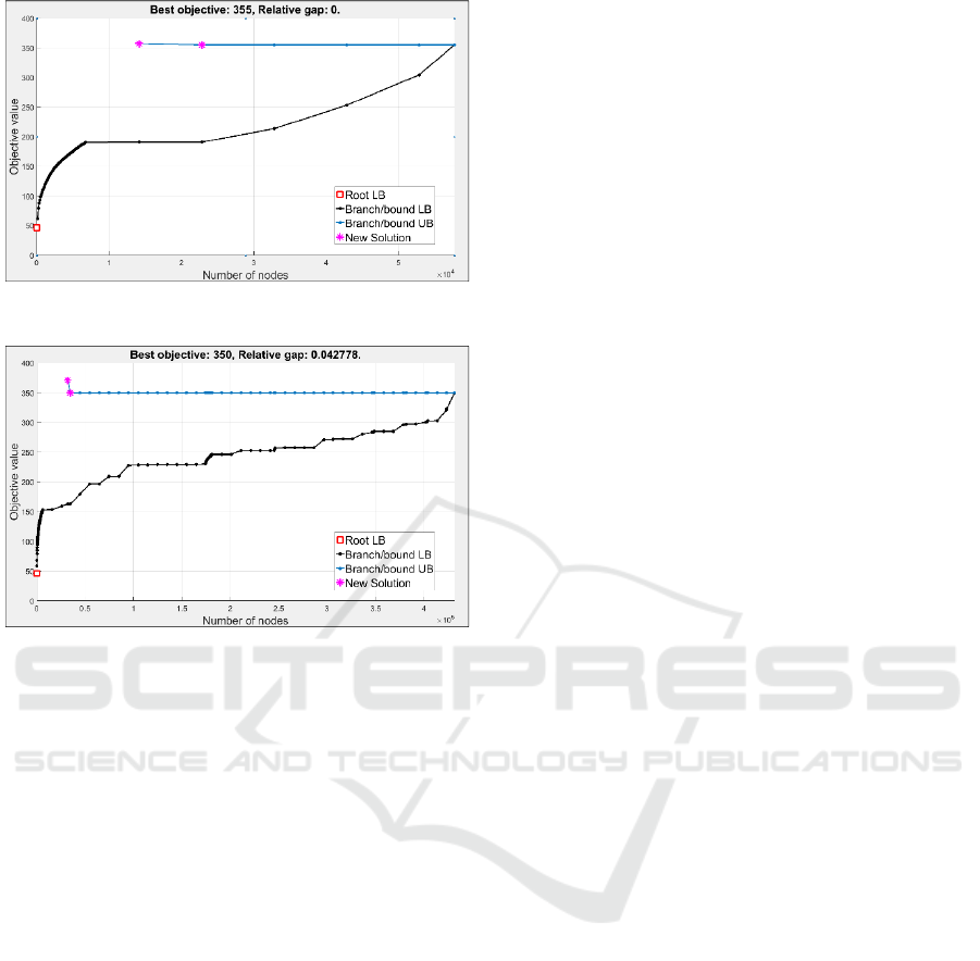
Figure 5: Convergence of 3 fixture/12 part problem.
Figure 6: Convergence of 4 fixture/12 part problem.
The sample problem size was not large. This was
due to limitations that resulted from both the
variable size increase and the solution time increase
for larger problems.
The results show that the variable size increases
by a decreasing factor for the linearly increasing
number of parts on a constant number of fixtures
(logistical growth). This growth in variable size
resulted in an exponential growth in solution times.
A similar observation of logistical growth was made
for the variable sizes that increased due to a linearly
increasing number of fixtures for a constant number
of parts. However, the solution times for this case
appear to increase logistically as well; as opposed to
the previous case, where solution times increased
exponentially.
The sharp growth in solution times from the
solver meant that limited fixture/part combinations
could be tested within a reasonable timeframe. As
the problem is NP-hard, it is expected that finding
exact solutions via the branch and bound algorithm
would be computationally expensive. The problem is
exasperated by the MATLAB® 2016a branch and
bound solver’s inability to utilise parallel processing
for this application, despite the multicore processor
of the machine used.
Optional parameters on the solver were adjusted
to yield solutions in minimum time. These included
the branch rule used (most fractional), node
selection criterion (minimum objective) and
algorithm used (primal-simplex), amongst others.
The tolerance parameters were also adjusted to cater
for the integer values used in the dataset.
The results from this sample problem set confirm
that the MILP model does create a schedule that
minimises the total idle time in the system. The
solver reached convergence for the sample set and it
was confirmed (by inspection) that the resultant
schedules from this algorithm were those of
minimum idle time.
4 CONCLUSIONS
This paper presented a three-stage procedure for the
optimal and combined scheduling of a synchronised
fixture and part manufacturing cell. The paper
focused on the third stage of the procedure where a
mixed integer linear programming (MILP) model
was used to optimally schedule the production
system The results demonstrated that the model
minimises the total idle time in the system, thus
saving on operating costs and tardiness penalties in
practice.
This is useful for mass customisation production
systems, where the use of reconfigurable fixtures in
the manufacturing process cannot be optimised with
conventional approaches.
Despite the logistical and exponential increases
in solution time (depending on which variable is
held constant – fixtures or parts), the MILP model is
valid for the production system described for a
problem of any reasonable size.
The MILP model is limited by the assumptions
listed in Section 3.3.2. Most of these are somewhat
redundant, as production systems would exhibit such
behaviour in most practical cases anyway. The unit
workflow requirement is a limiting factor, but this
could be edited to represent batch workflow quite
easily. The requirement that fixtures are already
made and waiting, is another limiting factor that is
not as readily solved.
Further work on this research topic involves
creating a heuristic to cope with larger-sized
problems more efficiently – producing sub-optimal
but good solutions with smaller variable sets and
reduced solution times. Other factors, such as the
influence of manufacturing new fixtures and
maintaining an optimal fixture inventory, can be
addressed in future research endeavours.
Optimal Scheduling of an on-Demand Fixture Manufacturing Cell for Mass Customisation Production Systems - Model Formulation,
Presentation and Validation
23

ACKNOWLEDGEMENTS
The financial assistance of the National Research
Foundation (NRF) towards this research is hereby
acknowledged (via the Blue Sky Research Grant:
91339). Opinions expressed and conclusions arrived
at are those of the authors, and are not necessarily to
be attributed to the NRF.
REFERENCES
Bi, Z.M. & Zhang, W.J., 2001. Flexible fixture design and
automation: Review, issues and future directions.
International Journal of Production Research, 39(13),
pp.2867–2894.
Choi, S.S., Cha, S.H. & Tappert, C.C., 2010. A Survey of
Binary Similarity and Distance Measures. Journal of
Systemics, Cybernetics & Informatics, 8(1), pp.43–48.
Fogliatto, F.S., da Silveira, G.J.C. & Borenstein, D., 2012.
The mass customization decade : An updated review
of the literature. International Journal of Production
Economics, 138(1), pp.14–25.
Groover, M.P., 2001. Chapter 15: Group Technology and
Cellular Manufacturing. In Automation, Production
Systems, and Computer-Integrated Manufacturing.
West Conshohocken, PA: Prentice-Hall, pp. 420–459.
Smith, S., Jiao, R. & Chu, C.H., 2013. Editorial: Advances
in mass customization. Journal of Intelligent
Manufacturing, 24(5), pp.873–876.
Thörnblad, K., Strömberg, A., Patriksson, M. & Almgren,
T., 2013. Scheduling optimization of a real flexible job
shop including side constraints regarding
maintenance, fixtures, and night shifts, Department of
Mathematical Sciences, Division of Mathematics,
Chalmers University and University of Gothenburg.
Wong, T.C., Chan, F.T.S. & Chan, L.Y., 2009. A
resource-constrained assembly job shop scheduling
problem with Lot Streaming technique. Computers
and Industrial Engineering, 57(3), pp.983–995.
Yao, X. & Lin, Y., 2016. Emerging manufacturing
paradigm shifts for the incoming industrial revolution.
The International Journal of Advanced Manufacturing
Technology, 85(5), pp.1665–1676.
Yu, J.M., Doh, H.H., Kim, J.S., Lee, D.H. & Nam, S.H.,
2012. Scheduling for a Reconfigurable Manufacturing
System with Multiple Process Plans and Limited
Pallets/Fixtures. International Journal of Mechanical,
Aerospace, Industrial, Mechatronic and
Manufacturing Engineering, 6(2), pp.232–237.
ICINCO 2017 - 14th International Conference on Informatics in Control, Automation and Robotics
24
