Adaptive Predictive Controller for a Servo Drive – Actuator/Sensor
Failure Study Experiments
Dariusz Horla
Institute of Control and Information Engineering, Faculty of Electrical Engineering, Poznan University of Technology,
ul. Piotrowo 3a, 60-965, Poznan, Poland
Keywords:
Predictive Control, Actuator Failure, Sensor Failure, Robust System.
Abstract:
The paper considers the problem of predictive control with actuator or sensor failures. The problem is to
show in what configuration (i.e. for what prediction horizons) the adaptive generalized predictive control can
tolerate these failures, assuring similar performance in comparison with the case without failures. The results
are shown on the basis of experiments conducted on the laboratory stand with a servo drive coupled with
a mechanical backlash module to mimic actuator/sensor failures, and with a magnetic brake, to show the
performance in the case of occurrence of an unexpected load.
1 INTRODUCTION
In order to obtain knowledge concerning a model of
a plant, adaptive control (enabling automatic tuning
of controller parameters) can be used to improve con-
trol performance, using recursive identification algo-
rithms to obtain estimates in an on-line fashion.
Receding horizon strategy in controls and predic-
tive control are relatively new methods in industrial
process control, in which a repeated optimization is
performed at every sampling instant. Since optimiza-
tion procedures are usually iterative-based, then even
in the case of the Generalised Predictive Controller
(GPC) a computational load must be taken into ac-
count when implementing this control method in real-
time regime.
In the paper, the GPC controller implemented as
C-MEX S-function (Horla, 2016) is used to con-
trol the Modular Servo System of Inteco, using a
USB interface and LAPACK library to perform nec-
essary matrix computations in the case of actua-
tor/sensor failures, to verify the applicability of the
GPC method (or its robustness) against unmodelled
work regimes, such as imprecise measurements or un-
expected changes in control signal. In addition, the
case of brake failure, what mimics constant and unex-
pected load on the shaft, is also taken into considera-
tion.
It is of practical importance to know if the con-
trol system can tolerate any failures in its compo-
nents. The design-based approaches are to design the
controller in such a way, as to enhance its capability
of being robust against failures or uncertainty, as in
(Yang et al., 2000b; Yang et al., 2000a; Zuo et al.,
2010). On the other hand, in the paper (Mhaskar
et al., 2006) the authors do take predictivecontrol into
consideration, but to build a bank of controllers with
special switching law in the case of an identified fail-
ure. In this paper, it is the control system that has
been analyzed from the viewpoint of possible failures
and their impact on the control performance, result-
ing with the information concerning applicability of
the GPC method in such situations, and extending the
results presented in (Horla, 2016).
The experimental setup is a servo drive with
the FPGA-based controller, allowing hardware-in-
the-loop experiments, and enabling rapid prototyping
of control algorithms to evaluate their performance.
The experimental setup is described on the basis of
(Horla, 2013) and (Horla, 2016).
Section 2 shortly describes the experimental
setup, Section 3 gives model description and equa-
tions of the GPC controller, taken from (Horla, 2016).
Section 4 presents the results of the experiments, and
the last Section summarizes the whole paper.
2 EXPERIMENTAL SETUP
The Inteco’s experimental setup comprises the DC
motor (12V, 77W, 250mNm, speed 3000rpm, cur-
rent 4.7A), tachogenerator and inertia load (brass
cylinder, 2kg, diameter 66mm, length 68mm), as
shown in Figure 1 (Inteco, a), (Inteco, b). The DC
Horla, D.
Adaptive Predictive Controller for a Servo Drive – Actuator/Sensor Failure Study Experiments.
DOI: 10.5220/0006415105510558
In Proceedings of the 14th International Conference on Informatics in Control, Automation and Robotics (ICINCO 2017) - Volume 1, pages 551-558
ISBN: 978-989-758-263-9
Copyright © 2017 by SCITEPRESS – Science and Technology Publications, Lda. All rights reserved
551

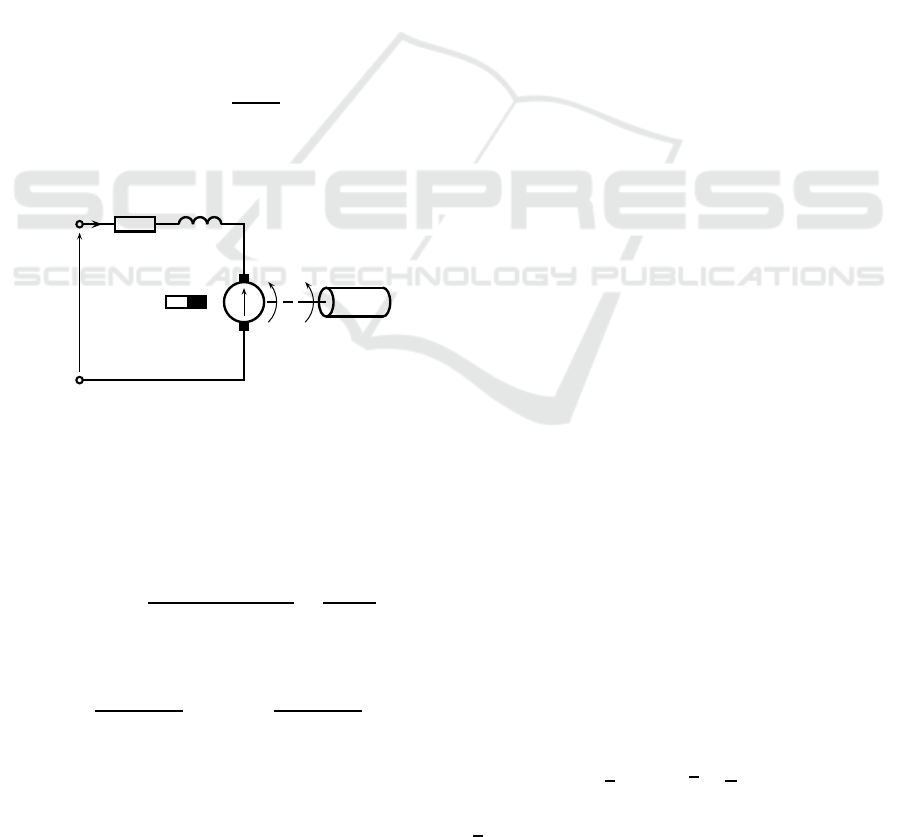
motor drives the inertia load and tachogenerator that
is connected directly to the DC motor, with voltage
proportional to the angular velocity, and y(t) =
˙
θ(t)
as its output. Additional modules of the laboratory
setup include encoder or magnetic brake modules.
The command input is fed to the servo drive from
an input-output card used by Real-Time Workshop
(MathWorks, 2015) and Simulink in order to work in
real-time regime. C-mex S-functions have been used
to implement the controller algorithm and estima-
tion scheme that has been downloaded to the FPGA
board. The control armature voltage e
a
(t) is limited
to ±12V, and is presented in the paper in dimension-
less form as |u(t)| ≤ 1.
The considered servo has the nonlinear static char-
acteristic related to the presence of a friction torque,
which has been compensated by its inverse, leading to
linear system equations (when no saturation occurs in
dynamic states) (Horla, 2013; Horla, 2016).
In accordance with (Horla, 2016), assuming the
following formula for the armature loop i
a
(t):
e
a
(t) = R
a
i
a
(t) + L
di
a
(t)
dt
+ e
m
(t) ,
constant flux and
e
m
(t) = k
e
˙
θ(t)
i
a
(t)
L
R
a
e
a
(t)
T(t) θ(t)
J, c
e
m
(t)
Figure 1: Diagram of experimental setup (Horla, 2013).
with the electromechanical torque T(t) = k
T
i
a
(t),
one gets
T(t) = J
¨
θ(t) + c
˙
θ(t).
Now, neglecting armature inductance, the ,,true”
continuous-time model transfer function becomes
G(s) =
k
T
R
a
Js+ R
a
c+ k
e
k
T
=
k
1+ sT
with:
k =
k
T
R
a
c+ k
e
k
T
, T =
R
a
J
R
a
c+ k
e
k
T
.
It is assumed that the ZOH-discretized model of
this plant is taken into consideration when implement-
ing the GPC algorithm with the sampling period of
T
S
= 0.1s.
3 PLANT MODEL
After linearization and assuming there is a noise cor-
rupting measurements, the model takes the form:
A(q
−1
)y
t
= B(q
−1
)u
t− d
+C(q
−1
)ξ
t
,
where u
t
and y
t
are input and output signals, respec-
tively, ξ
t
is assumed to be a white noise with zero
mean value and d is a dead time. The introduced poly-
nomials are given as:
A(q
−1
) = 1+ a
1
q
−1
+ a
2
q
−2
+ ... + a
nA
q
−nA
,
B(q
−1
) = b
0
+ b
1
q
−1
+ b
2
q
−2
+ ... + b
nB
q
−nB
,
C(q
−1
) = 1+ c
1
q
−1
+ c
2
q
−2
+ ... + c
nC
q
−nC
.
Since the GPC control enables tracking of a ref-
erence signal r
t
known N
y
samples in advance (Ca-
macho and Bordons, 1998), (Maciejowski, 2001), the
controller computes N
u
consecutive control signals, to
minimize the performance index given as
J =
Ny
∑
i=d
(r
t+ i
− ˆy
t+ i
)
2
+ q
u
Nu
∑
i=1
(∆v
t+ i−1
)
2
, (1)
where:
ˆy
t+ i
is an optimal i-step output prediction,
q
u
is a control signal weight,
N
u
and N
y
are control and prediction horizons, respec-
tively.
By solving the following Diophantine equations
(Camacho and Bordons, 1998):
∆A(q
−1
)E
i
(q
−1
) + q
−i
F
i
(q
−1
)=C(q
−1
), (2)
C(q
−1
)G
i
(q
−1
) + q
−i
Γ
i
(q
−i
)=E
i
(q
−1
)B(q
−1
), (3)
where i denotes output prediction step, the follow-
ing polynomials are obtained (nΓ = max(nB−1,nC−
1)):
E(q
−1
) = 1+ e
1
q
−1
+ ... + e
i−1
q
−i+1
,
F(q
−1
) = f
0
+ f
1
a
−1
+ ... + f
nA
q
−nA
,
Γ(q
−1
) = γ
0
+ γ
1
q
−1
+ ... + γ
nΓ
q
−nΓ
,
G(q
−1
) = g
0
+ g
1
q
−1
+ ... + g
i−1
q
−i+1
.
The polynomials introduced above enable one to
compute N
y
step output prediction as a sum of forced
and free responses:
ˆy
t+ 1
= G∆v
t
+ f
t+ 1
, (4)
where:
ˆy
t+ 1
=

ˆy
t+ 1
, ... , ˆy
t+ N
y

T
is the prediction of the
ICINCO 2017 - 14th International Conference on Informatics in Control, Automation and Robotics
552

output,
G is an impulse response matrix, i.e. with entries
from G
i
(q
−1
),
∆v
t
= [∆v
t
, ..., ∆v
t+ N
u
−1
]
T
is a computed control
signal vector,
f
t+ 1
=

ˆy
t+ 1/t
, .. ., ˆy
t+ Ny/t

T
is a free response vector.
In the unbounded case, and for (1), an explicit for-
mula for the control signal might be obtained:



∆u
t
= ∆v
t
=

G
T
G+ q
u
I

−1
G
T

r
t+ 1
− f
t+ 1

u
t
= ∆u
t
+ u
t− 1
.
(5)
When constraints become active u
t
6= v
t
, and con-
trol signal u
t
applied to the plant has a different am-
plitude than the computed control signal v
t
.
Since the Inteco Servo drive can be modeled as
the first-order inertia G(s) =
k
1+sT
in velocity con-
trol task, its discrete-time model is given with nA = 1,
nB = 0, d = 1, i.e.:
A(q
−1
) = 1− aq
−1
, B(q
−1
) = b.
From the solution of the Diophantine equations
with the assumed model, a sample form of prediction
(4) can be presented 3 steps ahead (a general rule can
be observed on this prediction):


ˆy
t+ 1
ˆy
t+ 2
ˆy
t+ 3


=


b 0 0
(a+ 1)b b 0
(a
2
+ a+ 1)b (a+ 1)b b




∆v
t
∆v
t+ 1
∆v
t+ 2


+
+


(a+ 1)y
t
− ay
t− 1
(a
2
+ a+ 1)y
t
− a(a + 1)y
t− 1
(a
3
+ a
2
+ a+ 1)y
t
− a(a
2
+ a+ 1)y
t− 1


that enables an easy way of generation of con-
trol signals according to (5). In addition, Γ
i
(q
−1
) =
γ
0
= 0, G
i
(q
−1
) = bE
i
(q
−1
), and it is assumed that
C(q
−1
) = 1.
The details of implementation in C code are given
in (Horla, 2016). The next section presents experi-
mental results obtained from the laboratory stand with
sampling period T
S
= 0.1s.
4 ACTUATOR/SENSOR FAILURE
CONSIDERATIONS
4.1 Preliminaries
All the to-be-presented experimental results have
been carried out in a fully adaptive system using the
on-line RLS identification scheme of the model of the
plant in the closed-loop system, with the initial es-
timates equal to half of their true values (identified
in a long time horizon for sufficiently exciting input
signal) and forgetting factor equal to unity (
˚
Astr¨om
and Wittenmark, 1989). The results are connected
with classical IAE and ISE performance indices cal-
culated on the basis of continuous-time signals from
the tracking system, being standard integrals of ab-
solute or squared tracking errors in the whole ex-
periment horizon (formulas omitted for the sake of
brevity). Every measurement set has been carried out
as a set of 55 experiments (all possible N
u
≤ N
y
con-
figurations), repeated 4 times, with mean values pre-
sented.
The following cases are taken into considera-
tion, when considering robustness of the GPC control
scheme of this plant to unmodelled situations:
• velocity sensor failure (mechanical backlash mod-
ule between brass cylinder and encoder),
• actuator failure (mechanical backlash module be-
tween DC motor and brass cylinder),
• brake failure (magnetic brake module included in
the system).
All the performance indices are presented as dif-
ferences between the case with the selected failure
model, and the nominal case with no failure (for
selected configuration of prediction horizons), both
in the sense of absolute value change and relative
(i.e. percentage) change – positive values refer to per-
formance deterioration, and negative – improvement.
4.2 Sensor Failure Results
As has been already remarked, the mechanical back-
lash unit has been connected in series between the DC
motor with brass cylinder module and the encoder, to
model sensor failure. In this way, any change in infor-
mation in dynamic states is generated by the encoder
when a full rotation of the shaft is made for the ve-
locity control task. With such a configuration of the
system, four series of measurements have been car-
ried out, in analogy to the series presented in (Horla,
2016).
As can be seen from Figure 2, the worst perfor-
mance deterioration takes place whenever N
u
and N
y
take on small values simultaneously, and the situation
improves with increasing N
y
. Performance indices for
N
y
= 10 are superior. In the case of percentage change
consideration, the intermediate performance deterio-
ration for larger N
y
results from small values of the
indices considered in experiments without failure. In
Figure 2(e), the results of a sample experiment have
Adaptive Predictive Controller for a Servo Drive – Actuator/Sensor Failure Study Experiments
553

been presented for the situation with and without ac-
tuator failure with the same configuration of the con-
troller.
The considered sensor failure model results in
poorer tracking during transients, but is of no mean-
ing in steady-state, i.e. for the stages with constant
reference signal. In the adaptive system, it results in
oscillatory behaviour of the closed-loop system, im-
proving performance of the identification algorithm.
It turns out that when failure of this kind takes
place, the best strategy is to keep a relatively long N
y
and short N
u
, this way the control action is mostly
abrupt, allowing faster transients. In the case of
longer N
u
horizon, the expected change in control sig-
nal extends over a number of samples, deteriorating
the performance during reverse of the shaft.
4.3 Actuator Failure Results
After connecting the mechanical backlash between
the DC motor and the brass cylinder, the system with
actuator failure model has been obtained. In this con-
figuration, the greatest absolute increase of perfor-
mance indices is observed for N
u
= N
y
= 1, i.e. in
one-step predictive controller. The situation improves
with increasing N
y
. To the great surprise, for N
u
= 1
and N
y
= 10 the both performance indices improved
in comparison with failure-free situation.
As can be seen from Figure 3, the considered ac-
tuator failure had no impact again on the steady-state
performance, but on increasing the dominating time
constant of the closed-loop system. The system was
slower, since it was impossible to change the velocity
of the shaft fast enough during reverse working mode,
due to the backlash.
Similar conclusions apply here as in the case of
the considered model of the sensor failure – the shaft
rotates faster leading to transfer the generated torque
sooner, as in the case of low-velocity rotation.
4.4 Brake Failure
In order to conduct this part of experiments, the lab-
oratory setup hitherto considered had to be modified,
and between the magnetic brake has been included the
brass cylinder and the encoder. During rotation, due
to Faraday’s law of induction, the current is induced
which magnetic fields generate load torque, accord-
ing to Lenz’s law. In this part, only two measuring se-
ries havebeen performedeach composed of 55 simple
measurements (see Fig. 4).
As expected, this situation must be connected with
overall performance degradation, which is, however,
neglectful for small N
u
and large N
y
configuration. It
is inadvisable to choose both large horizons of control
and prediction, since the identified model is inaccu-
rate (it does not take the load into account).
By observing the tracking performance presented
in Figure 4(e), it can be said that brake failure (i.e. in-
troduction of braking past some failure) results in
changes with control signal, but it does not alter
closed-loop system dynamics excessively.
Surprisingly, in the case of unexpected automatic
brake failure, already twice-mentioned configuration
of prediction horizons, enables one to improve the
control performance, by getting slower transients and
in this way, filtering-out of possible oscillations in the
error signal.
5 SUMMARY
The paper analyzed the situation of failures of the
control system and their impact on predictive con-
troller behaviour in such cases, to obtain a reliable
control system. It was interesting to verify if the GPC
scheme can tolerate any failures either in actuator or
sensor, thus this analysis was basically of practical in-
terest, enforced by presenting the results from a real
laboratory stand. In the future, it would be interesting
to verify if the sampling period allow one to obtain
any better improvement or reliability of the control
system.
ACKNOWLEDGEMENTS
The author wishes to thank to Mr. Pawel Szczygiel for
his help with performing necessary measurements.
REFERENCES
˚
Astr¨om, K. and Wittenmark, B. (1989). Adaptive Control.
Addison-Wesley.
Camacho, E. and Bordons, C. (1998). , Model Predictive
Control, pages 51–83. Springer.
Horla, D. (2013). Minimum variance adaptive control of
a servo drive with unknown structure and parame-
ters. Asian Journal of Control, DOI:10.1002/asjc.479,
15(1):120–131.
Horla, D. (2016). C-code implementation of an adaptive
real-time GPC velocity controller for a servo drive. In
Proceedings of the 17th International Conference on
Mechatronics, pages 1–6.
Inteco. Modular Servo System USB version Installation
Manual. Inteco.
Inteco. Modular Servo System User’s Manual. Inteco.
ICINCO 2017 - 14th International Conference on Informatics in Control, Automation and Robotics
554

Maciejowski, J. (2001). Predictive Control with Con-
straints. Pearson, UK.
MathWorks (2015). Real-time Workshop User’s Manual.
MathWorks.
Mhaskar, P., Gani, A., and Christofides, P. (2006). Fault-
tolerant control of nonlinear processes: Performance-
based reconfiguration and robustness. In American
Control Conference.
Yang, G.-H., Wang, J., and Soh, Y. (2000a). Reliable lqg
control with sensor failures. IEE Proceedings – Con-
trol Theory and Applications, 147(4):433–439.
Yang, Y., Yang, G.-H., and Soh, Y. (2000b). Reliable con-
trol of discrete-time systems with actuator failures.
IEE Proceedings – Control Theory and Applications,
147(4):428–432.
Zuo, Z., Ho, D., and Wang, Y. (2010). Fault tollerant con-
trol for singular systems with actuator saturation and
nonlinear perturbation. Automatica, 46:569–576.
Adaptive Predictive Controller for a Servo Drive – Actuator/Sensor Failure Study Experiments
555

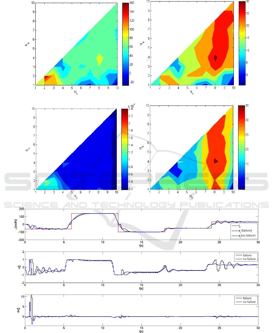
(a) Absolute IAE change (b) Relative IAE change (in %)
(c) Absolute ISE change (d) Relative ISE change (in %)
(e) Tracking performance with and without sensor failure, N
u
= 5, N
y
= 10
Figure 2: Experimental results concerning sensor failure with q
u
= 16,000, T
S
= 0.1s.
ICINCO 2017 - 14th International Conference on Informatics in Control, Automation and Robotics
556

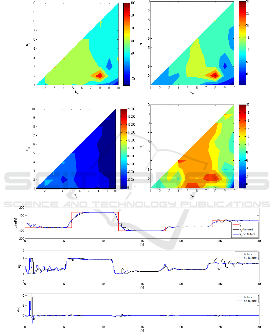
(a) Absolute IAE change (b) Relative IAE change (in %)
(c) Absolute ISE change (d) Relative ISE change (in %)
(e) Tracking performance with and without actuator failure, N
u
= 5, N
y
= 10
Figure 3: Experimental results concerning actuator failure with q
u
= 16,000, T
S
= 0.1s.
Adaptive Predictive Controller for a Servo Drive – Actuator/Sensor Failure Study Experiments
557

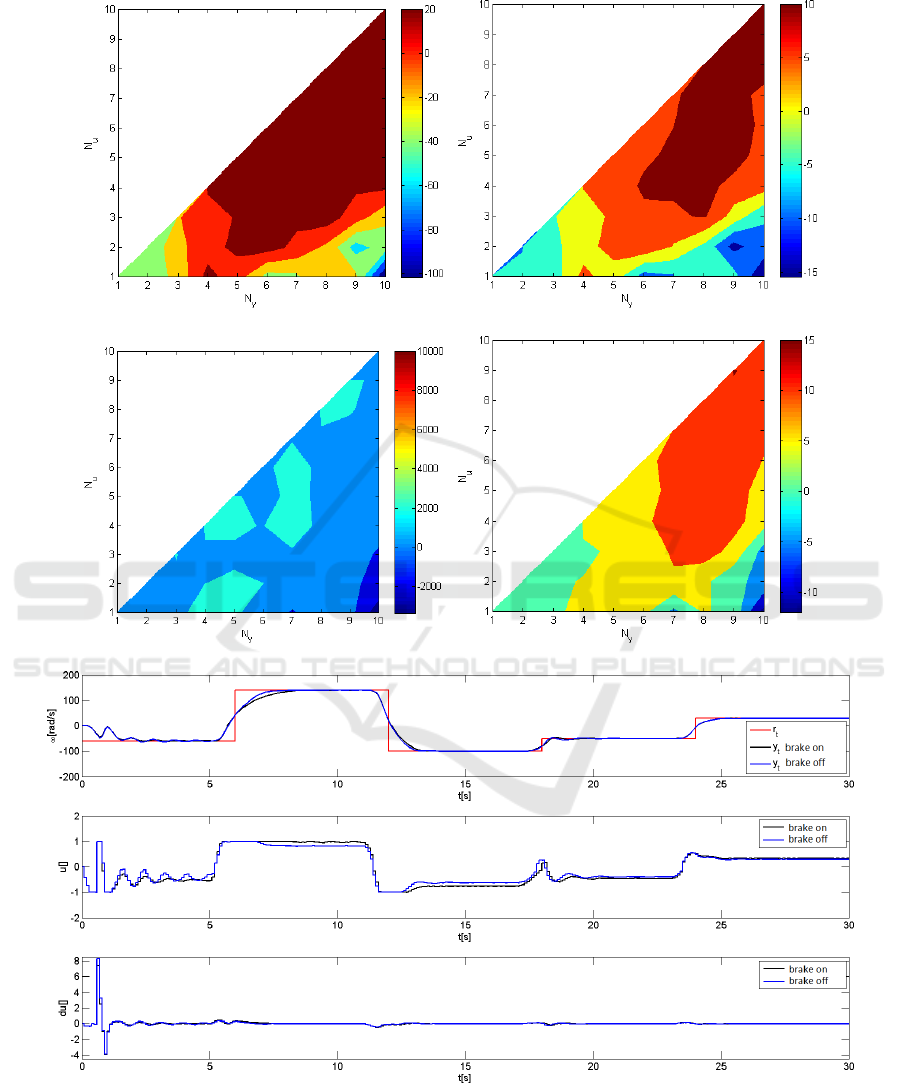
(a) Absolute IAE change (b) Relative IAE change (in %)
(c) Absolute ISE change (d) Relative ISE change (in %)
(e) Tracking performance with and without brake failure, N
u
= 5, N
y
= 10
Figure 4: Experimental results concerning brake failure with q
u
= 16,000, T
S
= 0.1s.
ICINCO 2017 - 14th International Conference on Informatics in Control, Automation and Robotics
558