Computational Burden Analysis for Integer Knapsack Problems Solved
with Dynamic Programming
Dariusz Horla
Institute of Control and Information Engineering, Faculty of Electrical Engineering, Poznan University of Technology,
ul. Piotrowo 3a, 60-965, Poznan, Poland
Keywords:
Optimization, Computational Burden, Dynamic Programming, Knapsack Algorithm.
Abstract:
The paper presents the results concerning computational burden analysis of dynamic programming and
bottom-up algorithms when solving knapsack problems. It presents the efficiency of the algorithms infor-
mation expressed both in calculation time, as well as mean number of iterations in knapsack problems up
to 15,000 items and capacity of the knapsack equal to 10,000. The aim of the paper is to present the this
knowledge what of practical use when solving optimization problems where estimate of execution time of the
algorithm is important.
1 INTRODUCTION
The knapsack problem (KP) is one of the most com-
mon, and at the same time, most interesting optimiza-
tion problems, which is defined as NP-hard (Kellerer
et al., 2004). The main assumptions are based on
maximizing the value of items in the knapsack with-
out exceeding its capacity. This task appears in col-
umn generation (CG) problem when solving optimal
1D cutting problem with dynamic programming and
is present in many engineering problems, e.g. choos-
ing the best strategy to select the most profitable
source of energy in the case of a demand (energy con-
sumption), constrained by some limits.
It appears, as remarked, in a cutting stock prob-
lem, and this paper aims at analysing further the com-
plexity of the presented algorithms.
In general, one can divide knapsack problems ac-
cording to two criteria. The first one is the dimen-
sionality of the problem (1D, 2D or 3D), and the sec-
ond one is the kind of the knapsack problem in accor-
dance to type of variables (discrete or continuous do-
main). In CG problems one encounters discrete knap-
sack problem with a single constraint, i.e. 1D knap-
sack problem.
In discrete/integer knapsack problems it is as-
sumed that it is impossible to include a fractional
value of the item to the knapsack, and their types can
be divided into: 0-1 knapsack problems, constrained
and unconstrained knapsack problems. In this paper,
the last case is considered, where the solution can in-
clude any feasible number of items, provided that the
maximum capacity is not exceeded. This problem has
the form (Moura, 2012)
max
x
c
T
x
s.t. w
T
x ≤ W ,
x ∈ Z
n
+
,
where c ∈ R
n
is the price vector, x ∈ R
n
is the vec-
tor comprising decision variables (number of items in
the solution), w ∈ R
n
is the weight vector (defining
weights of items), and W is the capacity of the knap-
sack.
2 SOLVING KNAPSACK
PROBLEMS
The following methods are crucial when solving 1D
knapsack problems: greedy algorithm and dynamic
programming. The first one is based on locally opti-
mal decisions made at every stage, what makes the
method easy to implement, but the obtained solu-
tion might not be globally optimal (Hristakeva and
Shrestha, 2005; Kellerer et al., 2004; Moura, 2012).
The first step of the algorithm is determination of
the price-to-weight ratio, i.e. h
i
=
c
i
w
i
, for every of n
items (variables), and in order to obtain the solution,
the items are selected in an orderly manner from the
highest to lowest value of h. On can formulate the
algorithm in four steps:
1) calculate h
i
for i = 1, . . ., n,
Horla, D.
Computational Burden Analysis for Integer Knapsack Problems Solved with Dynamic Programming.
DOI: 10.5220/0006415302150220
In Proceedings of the 14th International Conference on Informatics in Control, Automation and Robotics (ICINCO 2017) - Volume 1, pages 215-220
ISBN: 978-989-758-263-9
Copyright © 2017 by SCITEPRESS – Science and Technology Publications, Lda. All rights reserved
215

2) sort items with respect to descending values of h
i
,
set k = 1,
3) if the remaining capacity w
m,k
of the knapsack at
k-th stage of the algorithm exceeds the weight of
the i-th item, include this item x
i
= ⌊
w
m,k
w
i
⌋ times
(w
m,k
is the available capacity of the knapsack
when considering the k-th item); in the opposite
case, proceed to the next item and put k := k + 1,
4) repeat Step 3 until all items are considered.
Other types of greedy algorithm are not consid-
ered here, as e.g. (Ekel and Neto, 2006), sice the paper
is focused on giving background to the DP approach.
On the opposite to the greedy algorithm, there is a
brute force algorithm which generates all possible so-
lutions abiding constraints, and selecting the one for
which the objective function is maximized. It is easy
to implement, but at the same time is computationally
expensive, and can be formulated as follows:
1) generate matrix M ∈ R
m×n
of all (m) possible so-
lutions to the knapsack problem (put in rows),
2) generate vector r
comprising objective function
values for all rows of M,
3) find the maximum entry of r
, and set the corre-
sponding solution as optimal.
Dynamic programming (DP) is the method based
on successive division of the task into subproblems,
subproblems into subsubproblems, etc, proposed by
Richard Bellman, who was granted an IEEE medal in
1979 for this algorithm (Arora, 2004; Nocedal and
Wright, 1999; Randvidran et al., 2006). The next
stage is based on merging solutions to obtain the so-
lution of the initial problem. Every subproblem is
solved once only, what shortens the computation time,
and partial solutions are placed in the tableau (Moura,
2012; Kellerer et al., 2004). However, it may suffer
from the so-called curse of dimensionality for highly-
dimensioned problems (not discussed here).
In the case of the knapsack problem, the DP
tableau contains solutions for increasing capacity of
the knapsack in its last columns, and in subsequent
rows the number of available items is increased.
In the tableau (see Tab. 1), e.g. the entry P(1, 1)
is the largest objective function value for knapsack of
capacity equal to 1, with a one-element set of avail-
able items, P(n,W) is the largest objective function
for the knapsack with capacity of W and n avail-
able items. The optimal objective function value is
in P(n,W). In order to restore the values of decision
variables, the Bottom-Up algorithm must be used,
what will be given below.
The DP algorithm for the KP is summarized as
follows:
1) set initial values: P(0, 0) = 0, put P(0, j) = 0 ∀ j =
1, . . . , W and P(i, 0) = 0 ∀i = 1, . . . , n;
2) for consecutive capacities j = 1, . . . , W proceed
to Step 3;
3) for consecutive items i = 1, . . . , n proceed to Step
4;
4) if it holds that j ≥ w
i
, then put P(i, j) =
max(P(i− 1, j), P(i, j − w
i
) + c
i
), and, in the op-
posite case, put P(i, j) = P(i− 1, j);
5) repeat Step 2 until i = n ∩ j = W.
The Bottom-Up algorithm of restoring decision
variables in the optimal solution is as follows:
1) assume the initial entry to be P(n,W) and put i :=
n, j := W;
2) for P(i, j) = P(i− 1, j) put i := i− 1; in the oppo-
site case, put j := j − w
i
and update x
by substi-
tuting x
i
:= x
i
+ 1;
3) repeat Step 2 until P(i, j) 6= 0.
3 EXAMPLES
3.1 Greedy Algorithm
As an example of the greedy algorithm one can give
the following KP problem:
max
x
2x
1
+ x
2
+ x
3
+ 3x
4
+ x
5
+ x
6
+ 4x
7
+ 2x
2
+ x
9
s.t. 5x
1
+ 3x
2
+ 2x
3
+ 3x
4
+ 4x
5
+ 3x
6
+ 3x
7
+
+3x
8
+ 5x
9
≤ 14,
x
∈ Z
9
+
.
The following tableau presents the data of the problem:
i
1 2 3 4 5 6 7 8 9
w
i
5 3 2 3 4 3 3 3 5
c
i
2 1 1 3 1 1 4 2 1
h
i
0.40 0.33 0.50 1.00 0.25 0.33 1.33 0.67 0.20
.
By sorting the items with descending h
i
one gets (k =
1):
i
7 4 8 3 1 2 6 5 9
h
i
1.33 1.00 0.67 0.50 0.40 0.33 0.33 0.25 0.20
⌊
14
w
i
⌋
4 4 4 7 2 4 4 3 2
.
The remaining capacity W
m,1
= 14 > w
7
= 3, thus
x
7
= 4. The current capacity W
m,2
= 14− 12 = 2 (k =
2).
i
4 8 3 1 2 6 5 9
h
i
1.00 0.67 0.50 0.40 0.33 0.33 0.25 0.20
⌊
2
w
i
⌋ 0 0 1 0 0 0 0 0
.
As the result, x
3
= 1. The remaining capacity W
m,3
=
0 – the algorithm terminates. The optimal solution
becomes:
x
∗
= [0, 0, 1, 0, 0, 0, 4, 0, 0]
T
,
f(x
∗
) = 17.
ICINCO 2017 - 14th International Conference on Informatics in Control, Automation and Robotics
216

Table 1: DP tableau.
i-th item
price
i-th item
weight
No. of the
i-th item
Capacity j
0 1 2 ·· · W
0 0 0 0 0 0
c
1
w
1
1 0 P(1, 1) P(1, 2) ·· · P(1,W)
c
2
w
2
2 0 P(2, 1) P(2, 2) ·· · P(2,W)
.
.
.
.
.
.
.
.
.
.
.
.
.
.
.
.
.
.
.
.
.
.
.
.
c
n
w
n
n 0 P(n, 1) P(n, 2) ·· · P(n,W)
3.2 Dynamic Programming Algorithm
The sample DP problem in a KP framework is given
as below:
max
x
11x
1
+ 7x
2
+ 5x
3
+ x
4
s.t. 6x
1
+ 4x
2
+ 3x
3
+ x
4
≤ 15,
x
∈ Z
4
+
.
Item no. 1 has the price c
1
= 11 and the weight
w
1
= 6, and item no. 2 – the price c
2
= 7 and the
weight w
1
= 4 etc. In the first step (see Tab. 2), the
DP tableau is created (L
i
denotes the number of the
item).
By performing all calculations according to the
DP algorithm, the DP tableau is obtained (see Tab. 3).
Initial stages of filling-in of the DP tableau:
• j = 2, i = 2: weight w
2
= 6 > j − 1 = 1, thus
P(2, 2) = P(1, 2) = 0,
• j = 2, i = 3: weight w
3
= 4 > j − 1 = 1, thus
P(3, 2) = P(2, 2) = 0,
• j = 2, i = 4: weight w
4
= 3 > j − 1 = 1, thus
P(4, 2) = P(3, 2) = 0,
• j = 2, i = 5: weight w
5
= 1 ≤ j − 1 =
1, thus P(5, 2) = max(P(4, 2), P(5, 1) + 1) =
max(0, 1) = 1,
• j = 3, i = 2: weight w
2
= 6 > j − 1 = 2, thus
P(2, 3) = P(1, 3) = 0,
• j = 3, i = 3: weight w
3
= 4 > j − 1 = 2, thus
P(3, 3) = P(2, 3) = 0,
• j = 3, i = 4: weight w
4
= 3 > j − 1 = 2, thus
P(4, 3) = P(3, 3) = 0,
• j = 3, i = 5: weight w
5
= 1 ≤ j − 1 =
2, thus P(5, 3) = max(P(4, 3), P(5, 2) + 1) =
max(0, 2) = 2,
• . . .
The optimal objective function equals 27, and in
order to retrieve optimal solution, the Bottom-Up al-
gorithm must be used:
• j = 15, i = 4, since P(4, 15) = P(3, 15), item no. 4
is not included in the optimal solution, putting i :=
i− 1,
• j = 15, i = 3, since P(3, 15) 6= P(2, 15), item no. 3
is included in the optimal solution, putting j :=
j − w
3
and x
3
= x
3
+ 1,
• j = 12, i = 3, since P(3, 12) = P(2, 12), another
item no. 3 is not included in the optimal solution,
putting i := i− 1,
• j = 12, i = 2, since P(2, 12) = P(1, 12), item no. 2
is not included in the optimal solution, putting i:=
i− 1,
• j = 12, i = 1, since P(1, 12) 6= P(0, 12), item no. 1
is included in the optimal solution, putting j :=
j − w
1
and x
1
:= x
1
+ 1,
• j = 6, i = 1, since P(1, 6) 6= P(0, 6), another
item no. 1 is not included in the optimal solution,
putting j := j − w
1
and x
1
:= x
1
+ 1,
• j = 0, i = 1, since P(1, 0) = 0, algorithm termi-
nates.
The optimal solution becomes:
x
∗
= [2, 0, 1, 0]
T
,
f(x
∗
) = 17.
4 COMPARISON OF
ALGORITHMS
4.1 Computation Time Comparison for
the Considered Algorithms
As the performance indicator of the considered meth-
ods, the computation time of the given algorithm has
been selected. The first of the carried out tests (Prob-
lem 1) was the comparison of calculations for algo-
rithms with the knapsack with the capacity of 25 and
number of available items from 5 to 16. The results
are presented in Figure 1 and are averaged over 100
feasible and randomly-generated problems.
As can be seen, for problems with lesser num-
ber of available items, i.e. up to 9, the greedy algo-
rithm was the fastest, but it was with no guarantee
that the solution found was actually global. For large
problems, i.e. from 10 available items and above,
the fastest was the DP algorithm. It can be said
Computational Burden Analysis for Integer Knapsack Problems Solved with Dynamic Programming
217

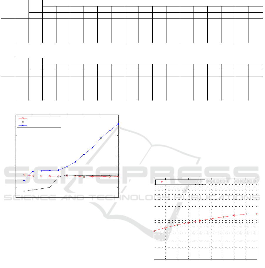
Table 2: Table in first step from the example.
c
i
w
i
L
i
Knapsack size j
0
1 2
3
4
5 6 7 8 9 10
11 12
13
14
15
0 0 0 0 0 0 0 0 0 0 0 0 0 0 0 0 0
11 6 1 0
7 4 2 0
6 3 3 0
1 1 4 0
Table 3: Final DP tableau from the example.
c
i
w
i
L
i
Knapsack size j
0
1 2
3
4
5 6 7 8 9 10
11 12
13
14
15
0 0 0 0 0 0 0 0 0 0 0 0 0 0 0 0 0
11 6 1 0 0 0 0 0 0 11 11 11 11 11 11 22 22 22 22
7
4 2 0 0 0 0 7 7 11 11 14 14 18 18 22 22 25 25
6
3 3 0 0 0 5 7 7 11 12 14 16 18 19 22 23 25 27
1
1 4 0 1 2 5 7 8 11 12 14 16 18 19 22 23 25 27
4 6 8 10 12 14 16
10
−4
10
−3
10
−2
10
−1
10
0
10
1
10
2
10
3
10
4
No. of variables
Solving time [s]
Solving time of a KP with capacity 25
Dynamic programming
Hasty algorithm
Brute force
Figure 1: Computation time of all considered algorithms.
that computation time in the case of the DP methods
does not change much with the number of available
items, what can be related to a relatively small num-
ber of both the items and the capacity of the knap-
sack. Another information is that brute force algo-
rithm solution times increases approximately expo-
nentially from 9 available items and above with in-
creasing number of available numbers. Thus it is only
the DP algorithm that is dedicated for large knapsack
problems, since the greedy algorithm does not guar-
antee one to obtain the global solution, and brute force
method is computationally expensive, e.g. the calcu-
lation time for 16 items too over 20 minutes!
Since the computation time for both brute force
and greedy algorithms does not depend on the ca-
pacity of the knapsack, the next results are related to
computation time for DP algorithm with respect to the
number of variables and varying capacity of the knap-
sack, where tests have been carried out for randomly
selected integer values of prices and demands.
Figure 2 depicts solution time for DP algorithm as
a function of number of decision variables for knap-
sack capacity of 15 (Problem 2). Despite the increase
in decision variables, mean calculation time remains
approximately the same, what is caused by very small
capacity of the knapsack with respect to the number
of variables. Secondly, the DP algorithm, on the con-
trary to the brute force method, might be successfully
implemented in problems with number of variables
exceeding 20.
5 10 15 20 25 30 35 40 45 50
10
−4
10
−3
10
−2
Solving time of a KP with capacity 15
No. of variables
Solving time [s]
Dynamic programming
Figure 2: Solution to Problem 2.
Figure 3 depicts solution time for DP algorithm as
a function of number of decision variables for knap-
sack capacity of 100 and maximum number of items
reaching 100 too (Problem 3). Once again, solution
time are approximately the same, what states that DP
algorithm is a good tool for solving such problems.
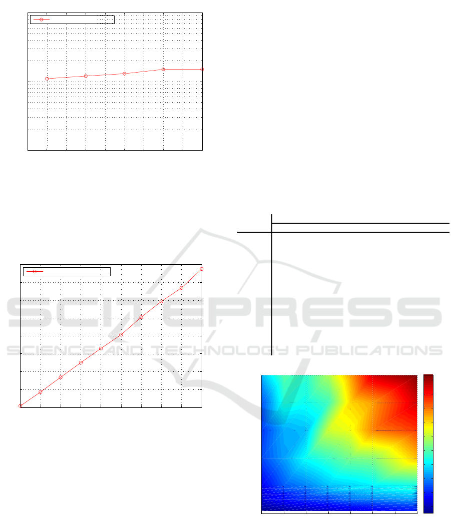
Figure 4 depicts solution time for DP algorithm as
a function of number of decision variables for knap-
sack capacity of 100 and maximum number of items
reaching 5,000 (Problem 4). Now, for a large num-
ber of items and large capacity of the knapsack, the
proper relation of solution time to available items can
ICINCO 2017 - 14th International Conference on Informatics in Control, Automation and Robotics
218

5 10 15 20 25 30 35 40 45 50
10
−4
10
−3
10
−2
Solving time of a KP with capacity 100
No. of variables
Solving time [s]
Dynamic programming
Figure 3: Solution to Problem 3.
be observed. This relation is approximately linear. In
addition to the latter, a single test for 15,000 items and
capacity of the knapsack equal to 10,000has been car-
ried out, giving solution reaching 109s. In practice,
however, such problems are rarely encountered.
500 1000 1500 2000 2500 3000 3500 4000 4500 5000
1
2
3
4
5
6
7
8
9
Solving time of a KP with capacity 10000
No. of variables
Solving time [s]
Dynamic programming
Figure 4: Solution to Problem 4.
5 ANALYSIS OF EFFICIENCY
5.1 Introduction
Since the number of iterations necessary to fill the
DP tableau can be easily calculated for every defined
problem (can be calculated only on the basis of the
size of the DP tableau). The mean number of iter-
ations of the Bottom-Up algorithm must be verified.
For the given capacity of the knapsack and available
items, random weight and price vectors have been
generated from a given range, and number of itera-
tions necessary to retrieve the values of the decision
variables has been identified. In order to improve the
accuracy of the performancetests, everyconfiguration
has been randomly generated 1,000 times, and results
have been averaged.
5.2 Results
The results have been presented in the tables below,
with corresponding plots included, in order to enable
better interpretation of the obtained results. The tests
have been carried out for the two following sets of
data:
• data set no. 1: the number of decision variables up
to 40 (see Tab. 4),
• data set no. 2: the number of decision variables
from 50 to 500 (see Tab. 5).
Table 4: Results for data set no. 1.
Capacity
No. of decision variables
5 10 15 20 25 30 40
10 10.63 15.25 18.65 22.78 27.75 32.10 40.85
20
15.53 21.39 25.31 28.87 33.56 36.69 42.62
30
18.69 26.54 32.16 34.33 40.21 41.60 48.60
40
21.88 31.06 37.09 41.35 47.04 50.03 56.75
50
26.64 35.08 43.25 46.71 55.62 57.34 65.22
60
27.86 38.24 45.87 50.25 60.66 64.13 71.49
70
26.07 35.51 49.99 57.51 62.78 68.26 76.26
80
30.54 46.28 51.41 66.72 68.22 75.27 81.08
90
27.00 48.87 55.33 66.50 79.24 75.11 91.40
100
31.91 51.37 59.70 71.52 75.31 80.67 87.69
200
47.28 64.64 84.44 94.23 105.7 109.1 144.9
300
44.07 67.06 70.67 122.7 129.6 156.1 171.2
400
49.40 89.36 85.67 95.81 139.6 150.8 190.3
500
69.69 99.52 91.78 116.2 150 189.8 207.1
5 10 15 20 25 30 35 40
0
50
100
150
200
250
300
350
400
450
500
Mean iteration count of the Bottom−Up algorithm, data set no. 1
No. of decision variables
Capacity
20
40
60
80
100
120
140
160
180
200
Figure 5: Mean iteration count of the Bottom-Up algorithm
(data set no. 1).
In the majority of cases, the increase in knapsack
capacity and increase in the number of decision vari-
ables, causes the mean number of iterations to in-
crease. This is easily interpretable, since the larger
the problem, the more iterations the algorithm must
perform.
Computational Burden Analysis for Integer Knapsack Problems Solved with Dynamic Programming
219

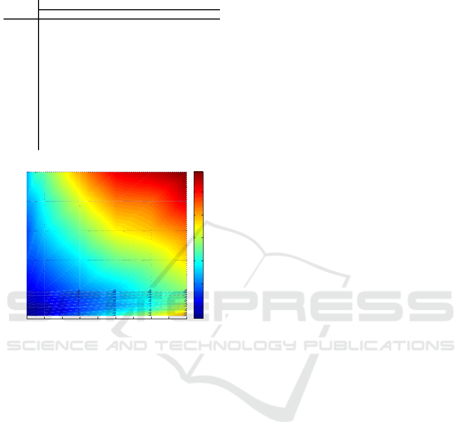
Table 5: Results for data set no. 2.
Capacity
No. of decision variables
50 75 100 200 300 400 500
10 52.67 75.74 100.7 200.8 299.7 400.0 499.7
20
49.76 72.15 91.94 187.0 279.5 381.1 476.7
30
55.84 72.06 86.34 155.9 252.1 315.9 430.6
40
64.46 77.13 95.25 170.7 221.5 303.1 426.0
50
71.96 88.56 101.7 156.7 216.7 284.7 396.2
60
79.85 93.74 108.8 164.3 240.0 304.9 379.6
70
84.08 104.1 116.5 174.9 225.0 296.1 358.6
80
92.15 112.4 128.4 177.8 233.5 305.4 367.9
90
101.2 119.7 133.9 192.2 238.3 313.4 339.6
100
103.0 125.7 138.3 209.0 252.4 319.0 383.5
200
168.3 177.2 201.6 278.0 352.3 389.1 464.4
300
169.4 225.2 261.1 354.1 447.3 479.7 531.6
400
224.2 253.6 299.3 426.6 523.9 539.2 628.6
500
233.7 330.8 350.2 504.3 618.3 646.3 687.5
50 100 150 200 250 300 350 400 450 500
0
50
100
150
200
250
300
350
400
450
500
Mean iteration count of the Bottom−Up algorithm, data set no. 2
No. of decision variables
Capacity
100
200
300
400
500
600
Figure 6: Mean iteration count of the Bottom-Up algorithm
(data set no. 2).
In the second table, the increase in knapsack ca-
pacity and in number of variables causes the number
of iterations of the Bottom-Up algorithm to increase.
However, for a large problem with 500 variables and
capacity equal to 500, the mean number of iterations
becomes 687.5, what verifies the applicability of the
dynamic programming algorithm here.
6 SUMMARY
It is important what the efficiency of the algorithms
used in solving, e.g. knapsack problems will be. This
paper aimed at giving the answer to this question for
problems with applicable dimensions, related to solu-
tions obtained in matter of seconds (if not – fractions
of a second) on a standard PC and Matlab. Results
presented in the figures related to mean number of it-
erations can be used easily to assess the time of calcu-
lations necessary to implement the algorithm on any
machine.
ACKNOWLEDGEMENTS
The author wishes to thank to Mr. Mateusz Pacek for
his help with formulating the benchmark problem.
REFERENCES
Arora, J. (2004). Introduction to optimum design. Elsevier,
2 edition.
Ekel, P. and Neto, F. S. (2006). Algorithms of discrete opti-
mization and their application to problems with fuzzy
coefficients. Information Sciences, 176(19):2846–
2868.
Hristakeva, M. and Shrestha, D. (2005). Different ap-
proaches to solve the 0/1 knapsack problem. In Pro-
ceedings of the 38th Midwest Instruction and Comput-
ing Symposium, pages 1–14. University of Wisconsin-
Eau Claire, Eau Claire, WI.
Kellerer, H., Pferschy, U., and Pisinger, D. (2004). Knap-
sack Problems. Springer.
Moura, L. D. S. (2012). An efficient dynamic programming
algorithm for the unbounded knapsack problem. Tech-
nical report, Universidade de federal de Rio Grande do
Sul, Porto Alegre.
Nocedal, J. and Wright, S. (1999). Numerical Optimization.
Springer.
Randvidran, A., Ragsdell, K., and Reklaitis, G. (2006).
Engineering optimization. Methods and applications.
Wiley, 2 edition.
ICINCO 2017 - 14th International Conference on Informatics in Control, Automation and Robotics
220