
Local Decay of Residuals in Dual Gradient Method Applied to MPC
Studied using Active Set Approach
Matija Perne, Samo Gerk
ˇ
si
ˇ
c and Bo
ˇ
stjan Pregelj
Jo
ˇ
zef Stefan Institute, Jamova cesta 39, Ljubljana, Slovenia
Keywords:
Model Predictive Control, Gradient Method, Optimization.
Abstract:
A dual gradient method is used for solving quadratic programs resulting from a model predictive control
problem in real-time control context. Evolution of iterates and residuals throughout iterations of the method
is studied. In each iteration, the set of active inequality constraints whose corresponding components of the
Lagrange multiplier are non-zero can be defined. It is found that the set of active constraints tends to stay
constant through multiple iterations. Observing the decay of residuals for intervals where the set of active
constraints is constant leads to interesting findings. For such an interval, the dual residual can be expressed in
a base so that its components are decaying independently, uniformly, and at predictable rates. The base and the
rates only depend on the system matrices and the set of active constraints. The calculated decay rates match
the rates observed in numerical simulations of MPC control, which is shown for the AFTI-16 benchmark
example.
1 INTRODUCTION
Model predictive control (MPC) is traditionally lim-
ited to processes with relatively slow dynamics be-
cause of the computational complexity of online op-
timization (Qin and Badgwell, 2003). In the last
decade, a considerable advance has been made in the
field of fast online optimization (Ferreau et al., 2008;
Wang and Boyd, 2010; Mattingley et al., 2011; Mat-
tingley and Boyd, 2012; Domahidi et al., 2012; Hart-
ley et al., 2014; Ferreau et al., 2014).
The advantages of MPC appear promising for
the implementation of advanced plasma current and
shape control in a tokamak fusion reactor (Gerk
ˇ
si
ˇ
c
and Tommasi, 2014). In particular, we are focusing
on fast online implementations of first-order methods
adapted for use with MPC (Richter, 2012; Gisels-
son, 2013; Kouzoupis, 2014; Giselsson and Boyd,
2015; Patrinos et al., 2015). Compared to active-set or
interior-point methods, they may require a consider-
able number of iterations to converge to the optimum.
However, each iteration is relatively simple, so that
the implementation is possible in restricted hardware,
and the methods were found to be computationally
efficient for the computation of quadratic programs
arising from MPC where a relatively low accuracy of
the solution is sufficient.
We are highly interested in complexity certifica-
tion, which proves that a solution with an acceptable
tolerance can be found in a certain maximum number
of iterations (limited time). However, useful certifica-
tion is currently not available for any of the relevant
methods in practical cases of control problems with
state constraints. Despite this, a number of methods
typically converge reasonably fast, hence our interest
in the practical rates of decay of residuals.
In this work, we examine the rates of decay of
residuals observed with a dual gradient method. In
our MPC simulations, we have observed very differ-
ent decay rates, which we found to be in close rela-
tion with the sets of constraints that were active in
the corresponding intervals. We present a theoretical
expression for the decay rates in intervals with a con-
stant set of active constraints, which can be computed
from the system matrices and the set of constraints.
The result is illustrated with MPC application to the
AFTI-16 control benchmark (Kapasouris et al., 1990;
Giselsson, 2013).
2 PROBLEM DESCRIPTION
2.1 MPC
Optimal control of a linear system with constraints
and with a quadratic cost in discrete time with finite
horizon N (Giselsson, 2013) is investigated. The dy-
54
Perne, M., Gerkši
ˇ
c, S. and Pregelj, B.
Local Decay of Residuals in Dual Gradient Method Applied to MPC Studied using Active Set Approach.
DOI: 10.5220/0006416500540063
In Proceedings of the 14th International Conference on Informatics in Control, Automation and Robotics (ICINCO 2017) - Volume 1, pages 54-63
ISBN: 978-989-758-263-9
Copyright © 2017 by SCITEPRESS – Science and Technology Publications, Lda. All rights reserved

namics is:
x(t + 1) = Ax (t) + Bu (t), (1)
where t is the time index, x is the system state, u is
the system input, the matrices A and B describe the
system dynamics. Value of x(0) is known. Possible
system states and inputs are constrained to x ∈ X , u ∈
U where X ⊂ R
l
, U ⊂ R
m
are polyhedra. A cost
function is defined:
J =
1
2
N
∑
k=0
(x
k
− x
ref
)
T
Q(x
k
− x
ref
)
+(u
k
− u
ref
)
T
R(u
k
− u
ref
)
(2)
where Q and R are symmetric positive semidefinite
cost matrices. Constant vectors x
ref
, u
ref
are reference
values.
The control is obtained by minimizing the cost
function J with respect to constraints
J
∗
= min
x
0
,...,x
N
,u
0
,...,u
N
J (x
k
, u
k
)
subject to x
k+1
= Ax
k
+ Bu
k
,
x
k
∈ X , u
k
∈ U,
x
0
= x(0). (3)
The question of finding the optimizer
(x
0
, . . . , x
N
, u
0
, . . . , u
N
) is a quadratic program
(QP) (Boyd and Vandenberghe, 2004). With the
receding-horizon implementation, u
0
is applied as
the current value of the controller output u(0).
2.2 Quadratic Program
We use the condensed form of the QP, in which only
u
k
are assembled into the optimization variable. The
x
k
-dependent terms of the cost function and the equal-
ity constraints corresponding to system dynamics are
substituted using (1) (Ullmann and Richter, 2012).
The QP (3) can thus be written as
minimize
1
2
z
T
Hz + c
T
z
subject to Cz b. (4)
The vector z ∈ R
k·m
is the optimization variable that
can be constructed as
z =
u
0
u
1
.
.
.
u
N
.
The Hessian H is symmetric positive semidefinite by
construction. We are particularly interested in exam-
ples with positive definite H, which is often the case.
Lagrange duality is used. Unconstrained optimization
minimize
1
2
z
T
Hz + c
T
z + v
T
Cz (5)
for constant value of vector v leads to the solution of
a related quadratic program with different constraints
(Everett, 1963)
minimize
1
2
z
T
Hz + c
T
z
subject to Cz b
0
. (6)
Lagrange multiplier v can be adjusted until b = b
0
and the solution of (5) solves the original problem (4).
Search for the correct value of Lagrange multiplier is
named solving the dual problem (Boyd and Vanden-
berghe, 2004).
2.3 Dual Proximal Gradient Method
Algorithm
The indicator function of the feasible set for d b,
g(d), is defined as
g(d) =
0; d b
∞; otherwise.
(7)
Its conjugate function g
∗
(d) is defined as
g
∗
(d) = sup
z
(d
T
z − g(z)). (8)
The iteration scheme is best described using proxim-
ity operator
prox
L
ψ
(d) = argmin
y
ψ(y) +
L
2
k
y − d
k
2
. (9)
The algorithm of the dual gradient method is
y
k
= argmin
z
1
2
z
T
Hz + c
T
z +
v
k
T
Cz
(10)
v
k+1
= prox
L
g
∗
v
k
+ Cy
k
, (11)
where gradient of the Lagrange dual function of the
objective function in (4) is Lipschitz continuous with
the constant L. The highest eigenvalue of M =
CH
−1
C
T
can always be used as L (Giselsson and
Boyd, 2014). By scaling C, L = 1 can be achieved,
so without loss of generality, L = 1 is assumed and
notation prox
1
g
∗
(d) = prox
g
∗
(d) is used.
It follows from the Moreau decomposition (Rock-
afellar, 1970, Theorem 31.5) (Giselsson and Boyd,
2014) that the prox operator of the conjugate of an
indicator function is
prox
g
∗
(d) = d − prox
g
(d). (12)
From definition of the proximity operator it follows
that prox
g
(d) is the projection of d onto the feasible
Local Decay of Residuals in Dual Gradient Method Applied to MPC Studied using Active Set Approach
55

set for d b, so it is a min operation and computa-
tionally inexpensive, rendering the whole (11) inex-
pensive. In addition, a closed form of the solution for
(10) exists:
y
k
= −H
−1
C
T
v
k
+ c
(13)
for every positive definite Hessian. Dual proximal
gradient method can thus be practically applied to
solving QPs of the form discussed in (4).
3 RATES OF DECREASE OF
RESIDUALS
We define active constraints in step k as those whose
corresponding components of v
k
are positive. The set
of these constraints is the active set in step k, labelled
ω
k
. The vector of the positive components of v
k
is la-
belled v
k
[ω
k
]. The matrix formed from the rows of C
that correspond to active constraints is labelled C[ω
k
].
The matrix formed from the intersections of the rows
and columns corresponding to active constraints of M
is M[ω
k
|ω
k
] and is a principal submatrix of M. It is
found that eigenvalues of M[ω
k
|ω
k
] determine the rate
of decrease of residuals.
Consider three iterations, k, k +1, k +2, for which
the active set remains constant (ω
k
= ω
k+1
= ω
k+2
=
ω). Let us define dual residuals
∆
k
= v
k+1
− v
k
(14)
∆
k+1
= v
k+2
− v
k+1
and analyse the relationship between ∆
k
and ∆
k+1
.
From(11), we get
v
k+1
= prox
g
∗
v
k
+ Cy
k
. (15)
According to (12),
v
k+1
= v
k
+ Cy
k
− prox
g
v
k
+ Cy
k
. (16)
Equation (16) combines with (13) into
v
k+1
= v
k
− Mv
k
− CH
−1
c
−prox
g
v
k
+ Cy
k
.
(17)
The components of ∆
k,k+1
that do not form ∆
k,k+1
[ω]
are equal to 0, so it is sufficient to study ∆
k,k+1
[ω]. By
definition of ω, (17) turns into
v
k+1
[ω] =
v
k
− Mv
k
− CH
−1
c − b
[ω] (18)
where we have taken into account that prox
g
(v
k
+
Cy
k
)[ω] = b[ω], following from the definition of ω.
Multiplying
v
k+1
[ω] = v
k
[ω] − M [ω|ω]v
k
[ω]
−
CH
−1
c + b
[ω]
(19)
follows. Definition (14) leads to
∆
k
[ω] = v
k+1
[ω] − v
k
[ω]. (20)
And, (19, 20) give
∆
k
[ω] = −M[ω|ω]v
k
[ω] −
CH
−1
c + b
[ω]. (21)
∆
k+1
can be expressed with ∆
k
:
∆
k+1
[ω] = −M [ω|ω]v
k+1
[ω]
−
CH
−1
c + b
[ω]
∆
k+1
[ω] = −M [ω|ω]
v
k
[ω] + ∆
k
[ω]
−
CH
−1
c + b
[ω]
∆
k+1
[ω] = ∆
k
[ω] − M [ω|ω]∆
k
[ω]
∆
k+1
[ω] = (I − M[ω|ω])∆
k
[ω], (22)
where I is the identity matrix the same size as
M[ω|ω].
Since M[ω|ω] is symmetric, its eigenvectors are
orthogonal (Graselli, 1975, p. 83) and (22) can be
conveniently diagonalized using eignedecomposition
into
d
k+1
= (I − D)d
k
. (23)
Here, D = V
T
M[ω|ω]V, d
k,k+1
= V
T
∆
k,k+1
[ω], V
is orthogonal and its columns are eignevectors of M,
D is diagonal with eigenvalues λ
ω
i
of M[ω|ω] on the
diagonal.
In each iteration, the i-th component of d
k
gets
multiplied by 1 − λ
ω
i
. If 0 < λ
ω
i
< 2, the component
is decreasing toward 0. It can be shown that the com-
ponents of v
k
that lie in the nullspace of M[ω|ω] do
not affect y
k
(see appendix). So, if λ
ω
i
= 0, the cor-
responding component does not influence the primal
solution y. Moreover, d
k
i
= 0 for λ
ω
i
= 0 if ω is a fea-
sible active set, as shown in the appendix. For a given
ω, the qudratic norm of residual is thus decreasing to-
ward 0 if 0 ≤ λ
ω
i
< 2 for every λ
ω
i
. The slowest com-
ponent of residual to decay corresponds to the lowest
non-zero λ
ω
i
; components of residual proportional to
higher λ
ω
i
have faster dynamics. If the ω being stud-
ied is the final active set and will not change in sub-
sequent iterations, the lowest non-zero λ
ω
i
determines
the convergence rate.
From theorem 4.3.15 in (Horn and Johnson, 1990)
it follows that the lowest eigenvalue of the symmetric
matrix M forms the lower bound for eigenvalues of
the principal submatrices M[ω|ω] of M, and the high-
est eigenvalue of M is the upper bound for eigenval-
ues of M[ω|ω]. M is positive semidefinite, so its low-
est eigenvalue is bigger or equal to 0. It has been as-
sumed that the highest eigenvalue of M is set below or
equal to 1 through multiplying C and b with a positive
constant. It guarantees convergence of the method for
ICINCO 2017 - 14th International Conference on Informatics in Control, Automation and Robotics
56

L = 1. Scaling the problem influences the local rate of
decrease of residual: enlarging M also enlarges each
M[ω|ω] and its eigenvalues, among them each lowest
non-zero eigenvalue that determines the local rate of
decrease of the slowest component of residual.
In MPC-related practical examples, the lowest
eigenvalue of M is typically equal to 0. The theo-
rem is thus not sufficient to derive a positive lower
bound for the lowest non-zero eigenvalue of the prin-
cipal submatrices M[ω|ω]. In particular, the lowest
non-zero eigenvalue of a principal submatrix M[ω|ω]
can be smaller than the lowest non-zero eigenvalue of
M.
It is worth noting that analysing eigenvalues of
M[ω|ω] for given ω is sufficient for determining the
local convergence rate. Convergence rate estimates
only depend on system matrices that are independent
of current MPC system state and reference. The vec-
tor of constraint limits b and the gradient c do not
influence the convergence rate directly, only through
ω.
4 PRACTICAL EXTENSIONS
4.1 Preconditioning or Generalization
Use of the generalized prox operator in place of the
prox operator can improve convergence (Giselsson,
2013). The generalized prox operator is defined in
the following way:
prox
L
µ
ψ
(d) = argmin
y
ψ(y) +
1
2
k
y − d
k
2
L
µ
, (24)
where L
µ
is chosen to be a diagonal positive definite
matrix. (11) is modified using the generalized prox
operator to obtain
v
k+1
= prox
L
µ
g
∗
v
k
+ Cy
k
. (25)
Consider the following quadratic program:
minimize
1
2
z
T
Hz + c
T
z
subject to
˜
Cz
˜
b, (26)
where
˜
C stands for EC and
˜
b is Eb, E being a di-
agonal positive definite matrix. Taking into account
(Giselsson, 2013)
prox
L
µ
g
∗
(d) = d − L
−1
µ
prox
L
−1
µ
g
(L
µ
d), (27)
it follows that using (10, 11) to solve (26) is equiva-
lent to solving (4) using (10, 25) if E = L
−1
µ
.
The procedure of generalization or precondition-
ing consists of finding a suitable E and changing the
QP in (4) into the one in (26). It is then solved us-
ing (10, 11). The matrix M is replaced by
˜
M =
˜
CH
−1
˜
C
T
= EME. The highest eignevalue of
˜
M is
chosen by scaling E and should be ≤ 1 for conver-
gence to be guaranteed taking L = 1. Better choices
of E lead to bigger lowest positive eigenvalues of the
encountered
˜
M[ω
k
|ω
k
].
4.2 Upper and Lower Boundaries
In MPC, it is typical to have upper and lower bounds
on the same signals, which leads to the same linear
functionals of the optimization variable in QP having
both upper and lower bounds as well. If the QP is
given in the form of (4), C can thus be written as
C =
C
1
−C
1
. (28)
Then inequality (4) can be reformulated as
b
1
C
1
z b
2
. (29)
In the computational code, C is replaced with C
1
, re-
sulting in smaller matrices (among them M) and in
halving the length of Lagrange multiplier, the same
component now corresponds to both the upper and the
lower boundary depending on its sign. It follows that
g(d) becomes the indicator function of the feasible set
for b
1
d b
2
. It causes prox
g
(d) to turn into pro-
jection onto a box that can be implemented using a
min and a max operation.
The modification does not change the theoretical
behaviour of the system but serves to lower the com-
putational needs. Importantly, rewriting (4) in the
form of (28) halves the size of M while keeping the
same eigenvalues of
˜
M[ω|ω] and preserving the rela-
tionship between
˜
M[ω|ω] and local rate of decrease
of residual. In the modified system, Lagrange multi-
plier components can be negative and constraints cor-
responding to negative components are included in ω.
4.3 Soft Constraints
QP resulting from an MPC problem with state con-
straints may not be feasible, meaning it does not nec-
essarily have a solution. However, in practice we
want the controller to produce a sensible output u also
when the constraints cannot be satisfied. One way to
achieve this is by relaxing the inequality state con-
straints from (4) with a slack variable which is penal-
ized in the cost function. The QP expands to the form
minimize
1
2
z
T
Hz + c
T
z + w
T
s (30)
subject to Cz b + s, (31)
Local Decay of Residuals in Dual Gradient Method Applied to MPC Studied using Active Set Approach
57

where s ∈ R
n
+
is the slack variable and w ∈ R
n
+
∪ ∞ is
its weight (Giselsson, 2013; Kouzoupis, 2014). If the
QP in (4) has a feasible solution and if the weight w
is big enough, the solution of the new problem is the
solution of the original QP and s = 0. For smaller w
or for infeasible QP, s has non-zero components.
A way to efficiently implement soft constraints
with linear cost of constraint violation can be seen by
comparing (5) to (30). If w is taken to be the upper
bound for Lagrange multipliers v, the dual proximal
gradient method solves the soft-constrained problem.
The components of the dual residual corresponding to
the violated soft constraints are 0, thus violated soft
state constraints appear among inactive constraints
when calculating the local rate of decrease of resid-
ual.
5 EXAMPLE
A discrete-time form of the AFTI-16 benchmark
model as in (Giselsson, 2013) has the system matri-
ces
A=
0.9993 −3.0083 −0.1131 −1.6081
−0.0000 0.9862 0.0478 0.0000
0.0000 2.0833 1.0089 −0.0000
0.0000 0.0526 0.0498 1.0000
B=
−0.0804 −0.6347
−0.0291 −0.0143
−0.8679 −0.0917
−0.0216 −0.0022
in (1). The constraints are:
X =
x ∈ R
4
;−0.5 − s
1
≤ x
2
≤ 0.5 + s
1
,
−100 − s
2
≤ x
4
≤ 100 + s
2
}
U =
u ∈ R
2
;−25 ≤ u
1
≤ 25,
−25 ≤ u
2
≤ 25
}
. (32)
The constraints on the components of x are soft, the
linear weight on the components of the slack is w =
[10
5
, 10
5
]
T
, and w
T
s(k) is added to the sum term in
(2). The cost matrices are
Q = diag(10
−4
, 10
2
, 10
−3
, 10
2
),
R = diag(10
−2
, 10
−2
). (33)
The reference x
r
is 0 in all components except for the
first 50 time steps of the simulation, during which x
4
is 10. Initial state at the beginning of the simulation is
x(0) = [0, 0, 0, 0]
T
.
A family of QP in condensed form (4) correspond-
ing to the MPC problem is formed for N = 10 using
QPgen (QPgen, 2014; Giselsson and Boyd, 2014).
The matrices C and H are constant while the vectors
b and c are dependent on the system state and the ref-
erence. The QPs are 20-dimensional (10 x 2 compo-
nents of u) with 40 lines in C (limits on 10 x 2 input
signals and 10 x 2 state components).
The preconditioning diagonal matrix E is chosen
so as to minimize the condition number of the non-
singular part of M while setting the highest eigen-
value of M to 1. QPgen finds E = diag(10.4796,
3.5413, 9.9973, 10.0080, 9.9987, 10.0005, 10.0000,
10.0037, 9.9990, 9.9997, 10.0001, 10.0033, 9.9989,
9.9979, 10.0003, 10.0036, 9.9999, 9.9965, 9.9972,
10.0034, 0.2058, 0.0918, 0.1003, 0.1000, 0.1007,
0.1001, 0.1005, 0.1000, 0.1004, 0.1001, 0.1007,
0.1000, 0.1004, 0.1001, 0.1009, 0.0999, 0.1004,
0.1000, 0.1013, 0.1000). The model is initially simu-
lated in closed loop with 10
6
iterations in every time
step for 100 time steps. The system state x is recorded
at every time step and used as the input initial state
for observing convergence of the resulting QPs. Al-
gorithm behaviour is analysed in all time steps for 1
to 3000 iterations.
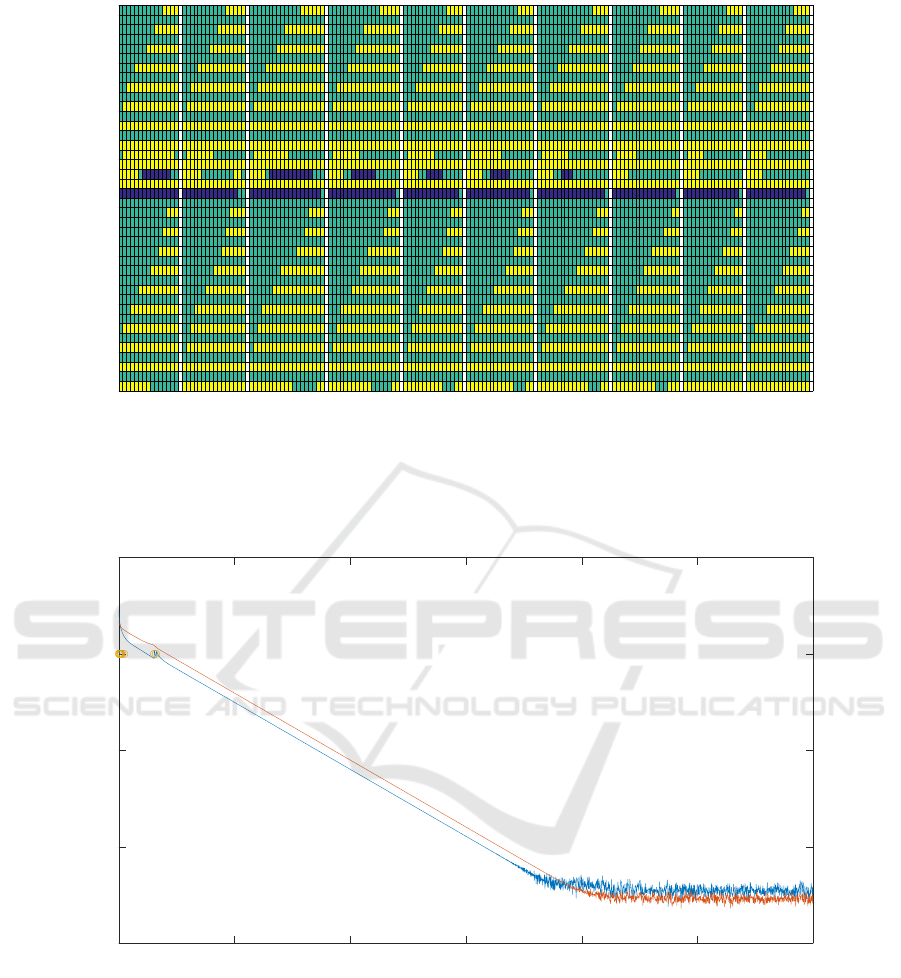
Figure 1 shows the active sets through iterations
for the first 10 time steps. White columns are delim-
iters of time steps.
In Figure 2, convergence through the active set
changes in time step 1 is shown graphically. Firstly
we analyse the behaviour with the final ω. The
quadratic norm of the primal residual is 0.22805 in
the 300th iteration and 8.74325×10
−12
in the 1800th
iteration, so the difference gets multiplied by 0.98414
in each iteration. This gives the estimate for the small-
est non-zero eigenvalue of the relevant M[ω|ω] of
1 − 0.98414 = 0.01586. In fact, 20 constraints are
active during the considered iterations (and no soft
ones are violated), 9 of them soft corresponding to
state constraints, and 11 hard corresponding to input
constraints. The matrix M[ω|ω] is non-singular and
its lowest eigenvalue is 0.01587, showing good agree-
ment with the numerical behaviour.
There is another longer interval in the first sam-
ple where the active set does not change between the
24th and 153rd iteration. The set has 22 elements, 9
of which are soft constraints and 13 are hard; no con-
straint is violated. If the dual residual is transformed
into the eigenspace of M[ω|ω], one expects the com-
ponents to decay in proportion with their correspond-
ing eigenvalues of M. These components are plotted
in Figure 3. It can be seen that the 22 lines decay
with different slopes in the relevant region and that the
ones listed higher in the legend decay slower. They
are listed in the figure in ascending order with respect
to eigenvalues (the first 2 correspond to the eigenval-
ues that are 0 and stay constant). Similarly, the active
set is constant from the 161st iteration on, has 20 ele-
ICINCO 2017 - 14th International Conference on Informatics in Control, Automation and Robotics
58
Active set number
20 40 60 80 100 120 140 160
Active set element
5
10
15
20
25
30
35
40
Figure 1: The list of active sets for the first 10 samples. The constraints are listed from the bottom to the top: the first 20
correspond to the input constraints on u from 1st to Nth time step, the following 20 are from constraints on x, again for 10
steps. Samples are listed from left to right with white columns separating them. For a given sample, the first active set is on
the left and every change of the active set results in a new column. Yellow fields mean active upper limit constraint. Blue
fields are for the lower limit. Green fields are inactive constraints or violated soft constraints.
Iteration
0 500 1000 1500 2000 2500 3000
Quadratic norm of residual
10
-15
10
-10
10
-5
10
0
10
5
Figure 2: Convergence of the quadratic norm of the primal (blue) and the dual (red) solution in time step 1 as a function of
the iteration number. The yellow circles mark iterations in which the active set changes.
ments, and M[ω|ω] has no eigenvalues equal to 0. The
corresponding eigendecomposition of the dual resid-
ual is shown in Figure 4.
Similar results for the time step 76 are shown in
Figures 5 and 6, and in 7 the non-transformed compo-
nents of the dual residual are shown for comparison.
For the majority of iterations, ω has 4 elements
and the lowest eigenvalue of M[ω|ω] is 0.1266 so
convergence is faster than in time step 1.
6 CONCLUSION
The different rates of convergence observed in nu-
merical simulations of the the dual gradient method
are explained with the theoretical computation of the
Local Decay of Residuals in Dual Gradient Method Applied to MPC Studied using Active Set Approach
59
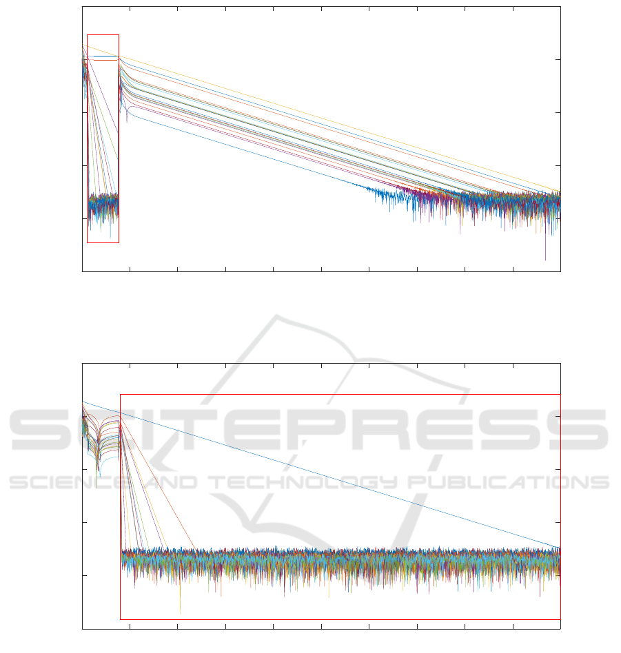
Iteration
0 200 400 600 800 1000 1200 1400 1600 1800 2000
Component of residual (iteration 24-153)
10
-20
10
-15
10
-10
10
-5
10
0
10
5
Figure 3: The components of the dual residual parallel to eigenvectors of M[ω|ω] between iterations 24 and 153 (red frame)
for time step 1 as a function of the iteration number. The components are listed in the order of ascending corresponding
eigenvalues.
Iteration
0 200 400 600 800 1000 1200 1400 1600 1800 2000
Component of residual (iteration 161+)
10
-20
10
-15
10
-10
10
-5
10
0
10
5
Figure 4: The components of the dual residual parallel to eigenvectors of M[ω|ω] from iteration 161 on (red frame) for time
step 1 as a function of the iteration number. The components are listed in the order of ascending corresponding eigenvalues.
local rate of decrease of residuals. The decay rates of
the residuals only depend on system matrices and the
active set on constraints and are independent of the
current MPC system state, the reference, and the limit
values of the constraints. For an active set ω, the de-
cay rate is limited by the lowest non-zero eigenvalue
of M[ω|ω]. The problem of certification can thus be
seen as seeking a lower bound for non-zero eigenval-
ues of M[ω|ω] for active sets ω that could possibly
occur.
In further work, we intend to test lower bounds
of as many active sets as possible, although it is gen-
erally known that this problem is plagued with com-
binatorial complexity. We will also try to extend the
approach to the fast dual gradient method without and
with restarting and use the results in the precondition-
ing phase to speed up convergence.
ICINCO 2017 - 14th International Conference on Informatics in Control, Automation and Robotics
60
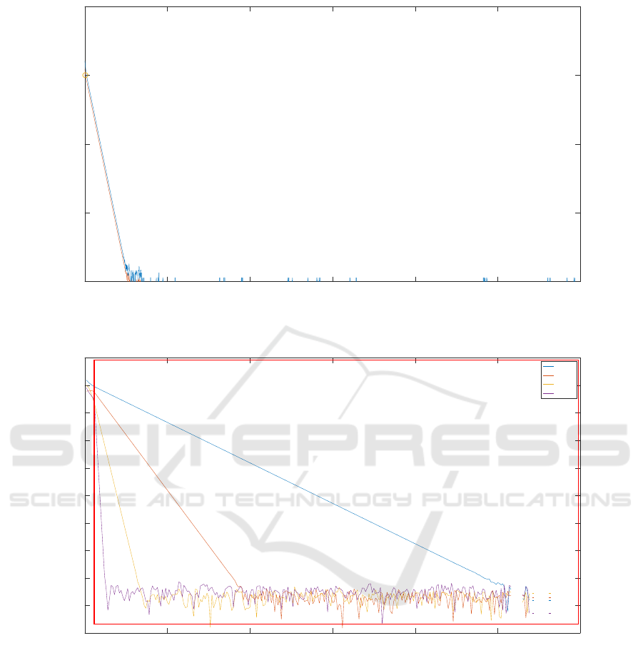
Iteration
0 500 1000 1500 2000 2500 3000
Quadratic norm of residual
10
-15
10
-10
10
-5
10
0
10
5
Figure 5: The quadratic norm of the primal (blue) and the dual (red) residual in time step 76 as a function of the iteration
number. The yellow circles mark iterations in which the active set changes.
Iteration
0 50 100 150 200 250 300
Component of residual (iteration 6+)
10
-18
10
-16
10
-14
10
-12
10
-10
10
-8
10
-6
10
-4
10
-2
10
0
10
2
data1
data2
data3
data4
Figure 6: The components of the dual residual parallel to eigenvectors of M[ω|ω] from iteration 6 on for time step 76 as a
function of the iteration number. The components are listed in the order of ascending corresponding eigenvalues.
ACKNOWLEDGEMENTS
Research supported by Slovenian Research Agency
(P2-0001). This work has been carried out within the
framework of the EUROfusion Consortium and has
received funding from the Euratom research and train-
ing programme 2014-2018 under grant agreement No
633053. The views and opinions expressed herein do
not necessarily reflect those of the European Commis-
sion.
REFERENCES
Boyd, S. and Vandenberghe, L. (2004). Convex Optimiza-
tion. Cambridge University Press, New York, NY,
USA.
Domahidi, A., Zgraggen, A. U., Zeilinger, M. N., Morari,
M., and Jones, C. (2012). Efficient Interior Point
Methods for Multistage Problems Arising in Reced-
ing Horizon Control. In Proceedings of the 51st IEEE
Conference on Decision and Control.
Everett, H. (1963). Generalized lagrange multiplier method
Local Decay of Residuals in Dual Gradient Method Applied to MPC Studied using Active Set Approach
61
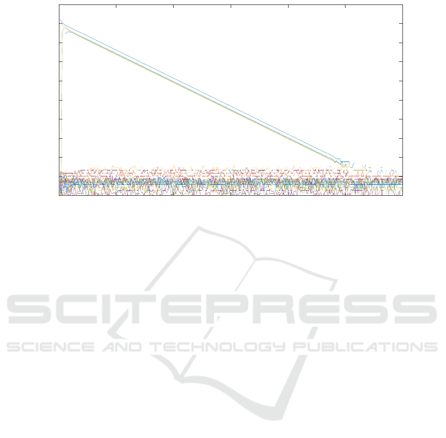
Iteration
0 50 100 150 200 250 300
Component of residual
10
-18
10
-16
10
-14
10
-12
10
-10
10
-8
10
-6
10
-4
10
-2
10
0
10
2
Figure 7: The original components of the dual residual for time step 76 as a function of the iteration number.
for solving problems of optimum allocation of re-
sources. Oper. Res., 11(3):399–417.
Ferreau, H. J., Bock, H. G., and Diehl, M. (2008). An on-
line active set strategy to overcome the limitations of
explicit MPC. International Journal of Robust and
Nonlinear Control, 18(8):816–830.
Ferreau, H. J., Kirches, C., Potschka, A., Bock, H. G., and
Diehl, M. (2014). qpoases: a parametric active-set al-
gorithm for quadratic programming. Math. Program.
Comput., 6(4):327–363.
Gerk
ˇ
si
ˇ
c, S. and Tommasi, G. D. (2014). Improving mag-
netic plasma control for ITER. Fusion Engineering
and Design, 89(910):2477 – 2488. Proceedings of
the 11th International Symposium on Fusion Nuclear
Technology-11 (ISFNT-11) Barcelona, Spain, 15-20
September, 2013.
Giselsson, P. (2013). Improving Fast Dual Ascent for MPC
- Part II: The Embedded Case. ArXiv e-prints.
Giselsson, P. and Boyd, S. (2014). Preconditioning in fast
dual gradient methods. In 53rd IEEE Conference on
Decision and Control, CDC 2014, Los Angeles, CA,
USA, December 15-17, 2014, pages 5040–5045.
Giselsson, P. and Boyd, S. (2015). Metric selection in fast
dual forward-backward splitting. Automatica, 62:1–
10.
Graselli, J. (1975). Linearna algebra. In Vi
ˇ
sja matematika
II. Dr
ˇ
zavna zalo
ˇ
zba Slovenije, Ljubljana, Slovenija.
Hartley, E. N., Jerez, J. L., Suardi, A., Maciejowski, J. M.,
Kerrigan, E. C., and Constantinides, G. A. (2014).
Predictive control using an FPGA with application to
aircraft control. IEEE Trans. Control Systems Tech-
nology, 22(3).
Horn, R. A. and Johnson, C. R. (1990). Matrix Analysis.
Cambridge University Press.
Kapasouris, P., Athans, M., and Stein, G. (1990). Design of
feedback control systems for unstable plants with sat-
urating actuators. In Proceedings of the IFAC Sympo-
sium on Nonlinear Control System Design, page 302
307. Pergamon Press.
Kouzoupis, D. (2014). Complexity of First-Order Methods
for Fast Embedded Model Predictive Control (Master
Thesis). Eidgenssische Technische Hochschule, Zrich.
Mattingley, J. and Boyd, S. (2012). CVXGEN: a code gen-
erator for embedded convex optimization. Optimiza-
tion and Engineering, 13(1):1–27.
Mattingley, J., Wang, Y., and Boyd, S. (2011). Receding
horizon control, automatic generation of high-speed
solvers. IEEE Control Syst. Mag., 31:52 –65.
Patrinos, P., Guiggiani, A., and Bemporad, A. (2015). A
dual gradient-projection algorithm for model predic-
tive control in fixed-point arithmetic. Automatica,
55(C):226–235.
Qin, S. and Badgwell, T. A. (2003). A survey of industrial
model predictive control technology. Control Engi-
neering Practice, 11(7):733 – 764.
QPgen (2014). QPgen. Accessed 24 January 2017.
Richter, S. (2012). Computational Complexity Certifica-
tion of Gradient Methods for Real-Time Model Pre-
dictive Control (Dissertation). Eidgenssische Tech-
nische Hochschule, Zrich.
Rockafellar, R. T. (1970). Convex Analysis. Princeton Uni-
versity Press, Princeton, New Jersey.
Ullmann, F. and Richter, S. (2012). FiOrdOs – MPC Ex-
ample. Automatic Control Laboratory, ETH Zurich,
Zurich.
Wang, Y. and Boyd, S. (2010). Fast model predictive control
using online optimization. IEEE Trans Control Syst
Techn, 18:267–278.
ICINCO 2017 - 14th International Conference on Informatics in Control, Automation and Robotics
62

APPENDIX
Components of v
k
Corresponding to
Nullspace of M[ω|ω] Do Not Influence y
k
Let M[ω|ω]v
ω
[ω] = 0. By definition,
M[ω|ω] = C[ω]H
−1
(C[ω])
T
. Since H
−1
is
positive definite, z
T
H
−1
z > 0 for every z dif-
ferent from 0 (Graselli, 1975, p. 90). Let z =
(C[ω])
T
v
ω
[ω]. Then 0 = (v
ω
[ω])
T
M[ω|ω]v
ω
[ω] =
(v
ω
[ω])
T
C[ω]H
−1
(C[ω])
T
v
ω
[ω] = z
T
H
−1
z. Thus
z = (C[ω])
T
v
ω
[ω] = 0. According to (13), addition
of v
ω
[ω] to v
k
[ω] does not affect y
k
.
Dual Residual Is Perpendicular to
Nullspace of M[ω|ω] for Feasible ω
If the definition of M[ω|ω] is taken into account in 21,
it follows:
∆
k
[ω] = −C [ω]H
−1
(C[ω])
T
v
k
[ω]
−C[ω]H
−1
c − b [ω]. (34)
Let t be a vector from nullspace of M[ω|ω]. Taking
the result from the previous appendix into account, it
follows (C[ω])
T
t = 0. Next, we calculate:
t
T
∆
k
[ω] = −t
T
C[ω]H
−1
(C[ω])
T
v
k
[ω]
−t
T
C[ω]H
−1
c − t
T
b[ω]
= −
(C[ω])
T
t
T
H
−1
(C[ω])
T
v
k
[ω]
−
(C[ω])
T
t
T
H
−1
c − t
T
b[ω]
= −t
T
b[ω].
If ω is a feasible active set, there exists a vector u so
that C[ω]u = b[ω]. Thus
t
T
∆
k
[ω] = −t
T
C[ω]u = −
(C[ω])
T
t
T
u = 0. (35)
An arbitrary vector t from the nullspace of M[ω|ω]
is orthogonal to ∆
k
[ω], so ∆
k
[ω] is orthogonal to the
nullspace of M[ω|ω].
Local Decay of Residuals in Dual Gradient Method Applied to MPC Studied using Active Set Approach
63
