
Initialization of Recursive Mixture-based Clustering with Uniform
Components
Evgenia Suzdaleva
1
, Ivan Nagy
1,2
, Pavla Pecherkov
´
a
1,2
and Raissa Likhonina
1
1
Department of Signal Processing, The Institute of Information Theory and Automation of the Czech Academy of Sciences,
Pod vod
´
arenskou v
ˇ
e
ˇ
z
´
ı 4, 18208, Prague, Czech Republic
2
Faculty of Transportation Sciences, Czech Technical University, Na Florenci 25, 11000, Prague, Czech Republic
Keywords:
Mixture-based Clustering, Recursive Mixture Estimation, Uniform Components, Bayesian Estimation.
Abstract:
The paper deals with a task of initialization of the recursive mixture estimation for the case of uniform com-
ponents. This task is significant as a part of mixture-based clustering, where data clusters are described by
the uniform distributions. The issue is extensively explored for normal components. However, sometimes the
assumption of normality is not suitable or limits potential application areas (e.g., in the case of data with fixed
bounds). The use of uniform components can be beneficial for these cases. Initialization is always a critical
task of the mixture estimation. Within the considered recursive estimation algorithm the key point of its initial-
ization is a choice of initial statistics of components. The paper explores several initialization approaches and
compares results of clustering with a theoretical counterpart. Experiments with real data are demonstrated.
1 INTRODUCTION
The use of mixture models is widespread in a range
of applications working with multi-modal systems re-
quiring to be described and identified (Hu et al., 2015;
Bao and Shen, 2016), for example, industry, fault de-
tection, transportation, marketing, medicine, etc. In
the field of data analysis, mixtures are used for model-
based clustering (Roy et al., 2017; Bouveyron and
Brunet-Saumard, 2014; Scrucca, 2016), where clus-
ters in the data space are described by distributions of
mixture components.
Various distributions are intensively investigated
for tasks of mixture-based clustering (Fern
´
andez et
al., 2016; Suzdaleva et al., 2015; Browne and McNi-
cholas, 2015; Morris and McNicholas, 2016). Gaus-
sian mixtures are probably the most frequently met
models, see, e.g., (Malsiner-Walli et al., 2016; Li et
al., 2016; O’Hagan et al., 2016), etc.
This paper considers a clustering with uniform
components of the mixture model. This is benefi-
cial for applications producing specific measurements
with fixed boundaries, where the assumption of nor-
mality or belongingness to the exponential family is
not suitable. A focus of the paper is a task of the mix-
ture initialization, which is known to be a critical part
of the mixture estimation significant for starting an
estimation algorithm.
Recent papers on the mixture initialization found
in the literature (Scrucca and Raftery, 2015; Mel-
nykov and Melnykov, 2012; Kwedlo, 2013; Shireman
et al., 2015; Maitra, 2009) are mostly concerned with
initialization of the expectation-maximization (EM)
algorithm (Gupta and Chen, 2011) used in iterative
approaches to mixture estimation. However, the ap-
proach discussed in the presented paper is based on
the recursive Bayesian estimation avoiding iterative
computations. It was considered for normal models
in (Peterka, 1981) and for normal mixtures in (K
´
arn
´
y
et al., 1998; K
´
arn
´
y et al., 2006; Nagy et al., 2011).
Extension of the approach for uniform components is
presented in (Nagy et al., 2016).
Within the mentioned framework, the initializa-
tion is primarily concerned with a choice of (i) the
number of components, (ii) the initial statistics of a
model of switching the components and (iii) the ini-
tial statistics of components. In this area, paper (Suz-
daleva et al., 2016) based on (K
´
arn
´
y et al., 2003) is
found, again devoted to the initialization with normal
mixtures.
This paper explores several initialization ap-
proaches for estimation of the mixture of uniform
components. The main emphasis is on the choice of
the initial statistics of components. The discussed me-
thods are based on the use of prior data and on a com-
bination of expert-based visualization techniques and
well-known clustering methods applied to prior data.
The paper is organized in the following way. Sec-
Suzdaleva, E., Nagy, I., Pecherková, P. and Likhonina, R.
Initialization of Recursive Mixture-based Clustering with Uniform Components.
DOI: 10.5220/0006417104490458
In Proceedings of the 14th International Conference on Informatics in Control, Automation and Robotics (ICINCO 2017) - Volume 1, pages 449-458
ISBN: 978-989-758-263-9
Copyright © 2017 by SCITEPRESS – Science and Technology Publications, Lda. All rights reserved
449

tion 2 introduces models and gives basic facts about
their individual estimation. Section 3 presents a brief
summary of recursive Bayesian estimation of mix-
tures of uniform components. Section 4 specifies the
initialization problem and considers four initialization
approaches. Section 5 provides results of their experi-
mental comparison. Conclusions and open problems
are given in Section 6.
2 MODELS
A considered system generates the continuous data
vector y
t
at each discrete time instant t = 1, 2,.....
The system is assumed to work in m
c
working modes.
Each of them is indicated at the time instant t by the
value of the unmeasured dynamic discrete variable
c
t
∈ {1, 2,... ,m
c
}, which is called the pointer (K
´
arn
´
y
et al., 1998).
For description of such the multi-modal system a
mixture model is used, which is here comprised of m
c
components in the form of the following probability
density functions (pdfs)
f (y
t
|Θ,c
t
= i), i ∈ {1, 2,. ..,m
c
}, (1)
where Θ = {Θ
i
}
m
c
i=1
is a collection of unknown
parameters of all components, and Θ
i
includes
parameters of the i-th component in the sense that
f (y
t
|Θ,c
t
= i) = f (y
t
|Θ
i
) for c
t
= i.
The general component pdf (1) is specified as the
uniform distribution. Under assumption of the inde-
pendence of individual entries of the vector y
t
(made
in this paper) the pdf (1) takes the following form
∀i ∈ {1, 2,. ..,m
c
}
f (y
t
|L,R, c
t
= i) =
(
1
R
i
−L
i
for y
t
∈ (L
i
,R
i
),
0 otherwise,
(2)
where {L
i
,R
i
} ≡ Θ
i
, and their entries (L
l
)
i
and (R
l
)
i
are minimal and maximal bounds of the l-th entry y
l;t
of the K-dimensional vector y
t
within the i-th uniform
component.
A component, which describes data generated by
the system at the time instant t is said to be active.
Switching the active components is described by a
model of the pointer c
t
as follows:
f (c
t
= i|c
t−1
= j,α) , i, j ∈ {1,2, ...,m
c
}, (3)
represented by the transition table
c
t
= 1 c
t
= 2 ·· · c
t
= m
c
c
t−1
= 1 α
1|1
α
2|1
·· · α
m
c
|1
c
t−1
= 2 α
1|2
·· ·
·· · ·· · ·· · ·· · ·· ·
c
t−1
= m
c
α
1|m
c
·· · α
m
c
|m
c
where a current value of the pointer corresponds to
the active component, and the unknown parameter α
is the (m
c
× m
c
)-dimensional matrix, and its entries
α
i| j
are non-negative probabilities of the pointer c
t
= i
(expressing that the i-th component is active at time t)
under condition that the previous pointer c
t−1
= j.
2.1 Individual Model Estimation
The estimation of parameters of the individual i-th
uniform component (2) in the case of independent
data entries is performed using the initially chosen
statistics L
t−1
and R
t−1
with the update of their l-th
entries for each l ∈ {1,...,K} in the following form,
see, e.g., (Casella and Berger, 2001):
if y
l;t
< L
l;t−1
, then L
l;t
= y
l;t
, (4)
if y
l;t
> R
l;t−1
, then R
l;t
= y
l;t
, (5)
where the subscript i is omitted for simplicity. The
point estimates of parameters are computed via
ˆ
L
t
= L
t
,
ˆ
R
t
= R
t
. (6)
According to (K
´
arn
´
y et al., 2006), parameter α of
the pointer model (3) is estimated using the conju-
gate prior Dirichlet pdf in the Bayes rule, recomput-
ing its initially chosen statistics and its normalizing.
The mentioned statistics is denoted by v
t−1
, which is
here the square m
c
-dimensional matrix. Its entries in
the case of available values c
t
= i and c
t−1
= j are
updated for i, j ∈ {1,. ..,m
c
} in the following way:
v
i| j;t
= v
i| j;t−1
+ δ(i, j; c
t
,c
t−1
), (7)
where δ(i, j; c
t
,c
t−1
) is the Kronecker delta function,
which is equal to 1, if c
t
= i and c
t−1
= j, and it is
0 otherwise. The point estimate of α is then obtained
by
ˆ
α
i| j;t
=
v
i| j;t
∑
m
c
k=1
v
k| j;t
. (8)
However, values of c
t
and c
t−1
are unavailable and
should be estimated. It means that generally for the
aim of the mixture-based clustering with the intro-
duced models it is necessary to estimate parameters
Θ and α and the pointer values.
3 UNIFORM MIXTURE
ESTIMATION
To specify a task of the mixture initialization, a neces-
sary theoretical background on recursive mixture es-
timation with uniform components should be given.
ICINCO 2017 - 14th International Conference on Informatics in Control, Automation and Robotics
450

The uniform distribution does not belong to the ex-
ponential family. Thus, extension of the general ap-
proach to recursive estimation (K
´
arn
´
y et al., 1998; Pe-
terka, 1981; K
´
arn
´
y et al., 2006; Nagy et al., 2011) for
this class of components is not straightforward and
might need the use of specific techniques of forget-
ting (Nagy et al., 2016).
Generally, the estimation algorithm is based on
using the joint pdf of unknown variables to be es-
timated and the Bayes and the chain rule (Peterka,
1981). The unknown parameters Θ and α (assumed
to be mutually independent) and the pointer values c
t
and c
t−1
enter the joint pdf as follows:
f (Θ, c
t
= i,c
t−1
= j,α|y(t))
| {z }
joint posterior pd f
∝ f (y
t
,Θ, c
t
= i,c
t−1
= j,α|y(t − 1))
| {z }
via chain rule and Bayes rule
= f (y
t
|Θ,c
t
= i)
|
{z }
(1)
f (Θ|y(t − 1))
| {z }
prior pd f o f Θ
× f (c
t
= i|α,c
t−1
= j)
| {z }
(3)
f (α|y(t − 1))
| {z }
prior pd f o f α
× f (c
t−1
= j|y(t − 1)),
| {z }
prior pointer pd f
(9)
∀i, j ∈ {1,2,...,m
c
}, where denotation y(t) =
{y
0
,y
1
,. .. ,y
t
} stands for the data collection up to the
time instant t, and y
0
denotes the prior information.
Recursive formulas for estimation of c
t
, Θ and
α are derived by marginalization of (9) over Θ, α
and c
t−1
. In the first case, the marginalization over
parameters Θ gives a closeness of the current data
item y
t
to individual components at each time in-
stant t, which is called the proximity, see, e.g., (Nagy
et al., 2016). Here, the normal approximation of
the uniform component, optimal in the sense of the
Kullback-Leibler divergence, see (K
´
arn
´
y et al., 2006),
is taken. It means that the proximity m
i
of the i-th
component is the value of the normal pdf obtained by
putting the point estimates of the expectation and the
covariance matrix of this uniform component from
the previous time instant t − 1 and the currently mea-
sured y
t
into
m
i
= (2π)
−K/2
|(D
t−1
)
i
|
−1/2
×exp
−
1
2
(y
t
− (E
t−1
)
i
)
0
(D
−1
t−1
)
i
(y
t
− (E
t−1
)
i
)
,
(10)
where K is a dimension of the vector y
t
, (E
t−1
)
i
is the
K-dimensional expectation vector of the i-th compo-
nent, each l-th entry of which is obtained via (6) as
follows:
(E
l;t−1
)
i
=
1
2
((
ˆ
L
l;t−1
)
i
+ (
ˆ
R
l;t−1
)
i
) (11)
and (D
t−1
)
i
is the covariance matrix containing on the
diagonal
(D
l;t−1
)
i
=
1
12
((
ˆ
R
l;t−1
)
i
− (
ˆ
L
l;t−1
)
i
)
2
. (12)
The proximities from all m
c
components comprise
the m
c
-dimensional vector m.
Similarly, the integral of (9) over α provides
the computation of its point estimate (8) using the
previous-time statistics v
t−1
.
However, the general purpose of the estimation is
to obtain the component weights (i.e., probabilities
that the components are currently active). For this
aim, the proximities (10) are multiplied entry-wise
by the previous-time point estimate of the parame-
ter α (8) and the prior weighting m
c
-dimensional vec-
tor w
t−1
, whose entries are the prior (initially chosen)
pointer pdfs (c
t−1
= j|y(t − 1)), i.e.,
W
t
∝
w
t−1
m
0
. ∗
ˆ
α
t−1
(13)
where W
t
denotes the square m
c
-dimensional matrix
containing pdfs f (c
t
= i,c
t−1
= j|y(t)) joint for c
t
and
c
t−1
, and .∗ is a “dot product” that multiplies the ma-
trices entry by entry. The matrix W
t
is normalized so
that the overall sum of all its entries is equal to 1, and
subsequently it is summed up over rows, which al-
lows to obtain the vector w
t
with updated component
weights w
i;t
for all components.
The maximal w
i;t
defines the currently active com-
ponent, i.e., the point estimate of the pointer c
t
at time
t. This point estimate is subsequently used for data
clustering.
3.1 The Statistics Updates
The above theoretical background leads to the fol-
lowing relations for updating the component statistics
(L
l;t−1
)
i
and (R
l;t−1
)
i
with the help of the obtained
weights w
i;t
at time t (Nagy et al., 2016). A specific
feature of the uniform component statistics is their
moving depending on a newly arrived data item. The
number of non-updates of each statistics is described
by the geometrical distribution. When the statistics is
not updated for a relatively long time, it is forgotten.
A scheme of forgetting is as follows. For the mini-
mum bound statistics (L
l;t−1
)
i
of the l-th entry of the
i-th component, the counter of its non-updates is set
as 0, i.e.,
(λ
L
l;t−1
)
i
= 0 (14)
Initialization of Recursive Mixture-based Clustering with Uniform Components
451

and then the update with forgetting takes the form
δ
L
= y
l;t
− (L
l;t−1
)
i
, (15)
if δ
L
< 0, (L
l;t
)
i
= (L
l;t−1
)
i
− w
i;t
δ
L
, (16)
(λ
L
l;t
)
i
= 0, (17)
else (λ
L
l;t
)
i
= (λ
L
l;t−1
)
i
+ 1, (18)
if (λ
L
l;t
)
i
> n, (L
l;t
)
i
= (L
l;t−1
)
i
+ φw
i;t
, (19)
where n is the allowed number of non-updates
computed from the distribution function of the ge-
ometrical distribution depending on the used confi-
dence interval and assumption of the statistics loca-
tion, see (Nagy et al., 2016), and φ is a small forget-
ting factor.
For the maximum bound statistics (R
l;t−1
)
i
the up-
date is performed similarly, i.e., (λ
R
l;t−1
)
i
= 0,
δ
R
= y
l;t
− (R
l;t−1
)
i
, (20)
if δ
R
> 0, (R
l;t
)
i
= (R
l;t−1
)
i
+ w
i;t
δ
R
,(21)
(λ
R
l;t
)
i
= 0, (22)
else (λ
R
l;t
)
i
= (λ
R
l;t−1
)
i
+ 1, (23)
if (λ
R
l;t
)
i
> n, (R
l;t
)
i
= (R
l;t−1
)
i
− φw
i;t
. (24)
3.2 The Pointer Update
The statistics of the pointer model is updated simi-
larly to the update of the individual categorical model
and based on (K
´
arn
´
y et al., 2006; K
´
arn
´
y et al., 1998),
but with the joint weights W
i, j;t
from the matrix (13),
where the row j corresponds to the value of c
t−1
, and
the column i to the current pointer c
t
v
i| j;t
= v
i| j;t−1
+W
j,i;t
. (25)
3.3 Algorithmic Summary
The briefly summarized above relations comprise the
following algorithmic scheme of clustering at each
time instant:
• Measuring the new data item;
• Computing the proximity of the data item to indi-
vidual components;
• Computing the probability of the activity of com-
ponents (i.e., weights) using the proximity, the
point estimate of the pointer model and the past
activity, where the maximal probability declares
the currently active component;
• Classifying data according to the declared active
component;
• Updating the statistics of all components and the
pointer model;
• Re-computing the point estimates of parameters
necessary for calculating the proximity.
4 MIXTURE INITIALIZATION
The main feature of the discussed recursive clustering
is its on-line performance and updating with each new
measurement. It is dangerous from the point of view
of the unsuccessful start of the algorithm, as it can
lead to dominance of one of the components. How-
ever, prior data sets, which are usually available in
most application areas (e.g., previous measurements,
realistic simulations, etc.) can be analyzed off-line for
the initialization purposes using a combination of rel-
atively simple expert-based techniques, e.g., (Suzdal-
eva et al., 2016) and well-known clustering methods
such as, e.g., k-means (Jain, 2010), etc.
The initialization task is specified for the above
recursive algorithm in the following way. For time
t = 0, ∀i, j ∈ {1, 2,...,m
c
} and for l ∈ {1,2,. .. ,K} it
is necessary to set:
• the number of components m
c
,
• the initial statistics of the pointer model v
i| j;0
and
the initial weighting vector w
0
,
• the initial components statistics (L
l;0
)
i
and (R
l;0
)
i
.
The last point is the key one. It is explained by com-
puting the proximity value, which depends on the pa-
rameter point estimates and, therefore, on the com-
ponent statistics. With the accurately chosen number
of components and the pointer statistics the proximity
with wrong initial component statistics leads to the
unsuccessful clustering.
4.1 Choice of Number of Components
Here a set of anonymized medical hematological prior
data is used for demonstration of the data visualiza-
tion with the aim of determining the number of com-
ponents. The following specific variables comprise
the 8-dimensional vector y
t
:
• y
1;t
– precollection number of leucocytes, [10
9
/l];
• y
2;t
– precollection number of HTK, [%];
• y
3;t
– precollection number of Hemoglobin (Hbg),
[g/dl];
• y
4;t
– precollection number of platelet count
(PLT), [10
9
/l];
• y
5;t
– precollection number of CD34+, [µl];
• y
6;t
– precollection number of CD34+ in total
blood volume (TBV), [10
6
],
• y
7;t
– concentration of mono-nuclear cells (MNC),
[%];
• y
8;t
– concentration of CD34+/kg, [10
6
].
ICINCO 2017 - 14th International Conference on Informatics in Control, Automation and Robotics
452
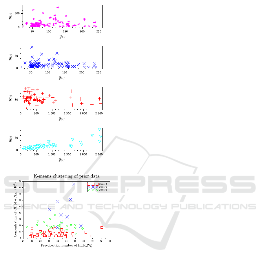
Figure 1: Visualization of selected prior data entries.
Figure 2: Three clusters detected by k-means in selected
prior data entries.
All the data entries are plotted against each other in
the form of upper triangular matrix of figures to de-
tect a number of visible clusters. If the visual analy-
sis is successful, and data clusters are distinguishable,
their number can be validated by using the k-means
method. To save space, selected data entries plotted
against each other are demonstrated in Figure 1. Two
bottom plots indicate that three clusters can be de-
tected, and they are also slightly distinguishable in the
two top plots. To verify the number of components,
the k-means is used, see Figure 2.
The initialized number of components can be also
validated by evolution of components weights during
the on-line estimation. This is demonstrated in Sec-
tion 5.
4.2 Initial Pointer Settings
The initial statistics of the pointer model v
i| j;0
and the
initial weighting vector w
0
are initialized either uni-
formly or randomly in combination with their upda-
ting by prior data.
4.3 Initial Components Statistics
Here four approaches to setting the initial statistics of
components are explored.
4.3.1 Component Centers via Mid-point Update
One of the approaches is to find centers of compo-
nents instead of the left and right bounds for initial de-
tection of components (Nagy et al., 2016). In this case
additional statistics should be used. They are (s
l;0
)
i
,
(q
l;0
)
i
, which are l-th entries of the K-dimensional
vectors s
t
and q
t
, where the last comprises a diago-
nal of a matrix. Starting from random values, they are
updated by a small set of prior data ∀i ∈ {1,2,... ,m
c
}
and ∀l = {1, .. ., K} in the following way.
(s
l;t
)
i
= (s
l;t−1
)
i
+ w
i;t
y
l;t
, (26)
(q
l;t
)
i
= (q
l;t−1
)
i
+ w
i;t
y
2
l;t
, (27)
After updating they are used to compute the point esti-
mates of the mid-point and mid-range vectors of each
component (S
t
)
i
and (h
t
)
i
respectively as follows.
(
ˆ
S
t
)
i
= (s
t
)
i
/t, (28)
(D
t
)
i
=
(q
t
)
i
− (s
t
)
i
(s
0
t
)
i
/t
/t, (29)
(
ˆ
h
t
)
i
=
p
3diag((D
t
)
i
), (30)
where (D
t
)
i
is the covariance matrix of the uniform
distribution, and
p
3diag((D
t
)
i
) denotes the square
roots of entries of the vector diag((D
t
)
i
). (28) and
(29) from the previous time instant are placed instead
of the expectation and the covariance matrix into the
proximity (10). In the end of updating by prior data
the mid-point (
ˆ
S
l;t
)
i
is the center of the i-th compo-
nent for the l-th data entry. The point estimates of the
minimum and maximum bounds are then obtained as
(
ˆ
L
l;t
)
i
= (
ˆ
S
l;t
)
i
− ε, (31)
(
ˆ
R
l;t
)
i
= (
ˆ
S
l;t
)
i
+ ε, (32)
with small ε, and they are used in (11) and (12) during
the on-line estimation according to Section 3.
4.3.2 Centers based on K-means
Another way is to use the centers of clusters initially
detected by the k-means method from prior data and
put them into (31) and (32) to be used during the on-
line estimation according to Section 3.
Initialization of Recursive Mixture-based Clustering with Uniform Components
453

4.3.3 Centers as Averages
The average values from individual prior data entries
with small deviations can be taken as initial centers of
components and then substituted into (31) and (32).
4.3.4 Bounds as Minimum and Maximum
Here the minimum and maximum values of corre-
sponding entries of the data vector y
t
are used directly
as the component statistics (L
l;0
)
i
and (R
l;0
)
i
respec-
tively. Then via (6) they enter (11) and (12).
4.3.5 Initialization Algorithm
This section presents Algorithm 1 tailored to the dis-
cussed initialization approaches. It is supposed to run
only with the available prior data set up to the time
instant t = T (where T is whole number of prior data)
before the on-line time loop of the clustering.
Finally, in the case of using Section 4.3.1, results
of Algorithm 1 are (
ˆ
S
l;T
)
i
, which is the center of the
i-th component for the l-th entry of y
t
, and the com-
ponent weights, both recursively updated by all prior
data. Results obtained according to Sections 4.3.2
and 4.3.3 are the component centers computed off-
line and the component weights. With the help of the
last technique from Section 4.3.4, the initial bounds
of components are obtained along with the weighting
vector.
For the on-line (i.e., for t = T + 1,T + 2,...) es-
timation of the component bounds and classification
of data among components according to the actual
maximum weight, the algorithm summarized in Sec-
tion 3.3 is applied. For the three first initialization
techniques, relations (31) and (32) should be used be-
fore measuring the first data item y
t
.
5 EXPERIMENTS
This section provides the experimental comparison of
the described initialization approaches with the help
of real data introduced in Section 4.1. The validation
of approaches was performed according to three fol-
lowing criteria:
• Evolution of component weights, which express
the activity of components, is observed during the
on-line estimation. The rare activity of some com-
ponent or its absence indicates that the number of
components is incorrectly initialized and proba-
bly too high. The regular activity of all compo-
nents validates the correct choice of the number
of components.
Algorithm 1.
{Preliminary initialization (for t = 0)}
Set the number of components m
c
.
for all i, j ∈
{
1,2, .. .,m
c
}
and l ∈
{
1,2 .. .,K
}
do
Set the initial random values of the component
mid-point and mid-range statistics (s
l;0
)
i
, (q
l;0
)
i
and the pointer statistics v
0
according to (26),
(27) and (25).
Using these statistics, compute the point esti-
mates (28), (29), (30) and (8).
end for
for all i ∈
{
1,2, .. .,m
c
}
do
Set the initial (random or uniform) weighting
vector w
0
.
end for
{Initialization with prior data set (for t = 1, .. .,T )}
for t = 1,2, .. .,T do
Load the prior data item y
t
.
for all i, j ∈
{
1,. .. ,m
c
}
and l ∈
{
1,. .. ,K
}
do
Obtain the proximities (10) as follows:
if According to Section 4.3.1, then
Use (28) and (29) in (10).
else if According to Section 4.3.2, then
Put the k-means centers in (31) and (32).
Compute (11), (12) and (10).
else if According to Section 4.3.3, then
Use means of data entries as (
ˆ
S
l;t
)
i
in (31)
and (32).
Compute (11), (12) and (10).
else if According to Section 4.3.4, then
Set (L
l;t
)
i
and (R
l;t
)
i
as minimum and max-
imum values of prior data entries.
Using (6), compute (11), (12) and (10).
end if
Using (10) and (8), compute the weighting
vector w
t
via (13), its normalization and sum-
mation over rows.
Update the pointer statistics (25).
Re-compute its point estimate (8).
if According to Section 4.3.1, then
Update the statistics (26), (27).
Re-compute the point estimates (28), (30)
and (29) and go to the first step of the ini-
tialization with prior data.
end if
end for
end for
• Evolution of the point estimates of component
parameters (i.e., bounds) is monitored at the be-
ginning of the on-line estimation. Fast locating
the stabilized values of the point estimates means
that the initialization is successful.
• The shape and the location of final clusters de-
ICINCO 2017 - 14th International Conference on Informatics in Control, Automation and Robotics
454
tected in the data space by starting the estimation
algorithm with the mentioned initialization tech-
niques are compared. Comparison with k-means
clustering is also demonstrated.
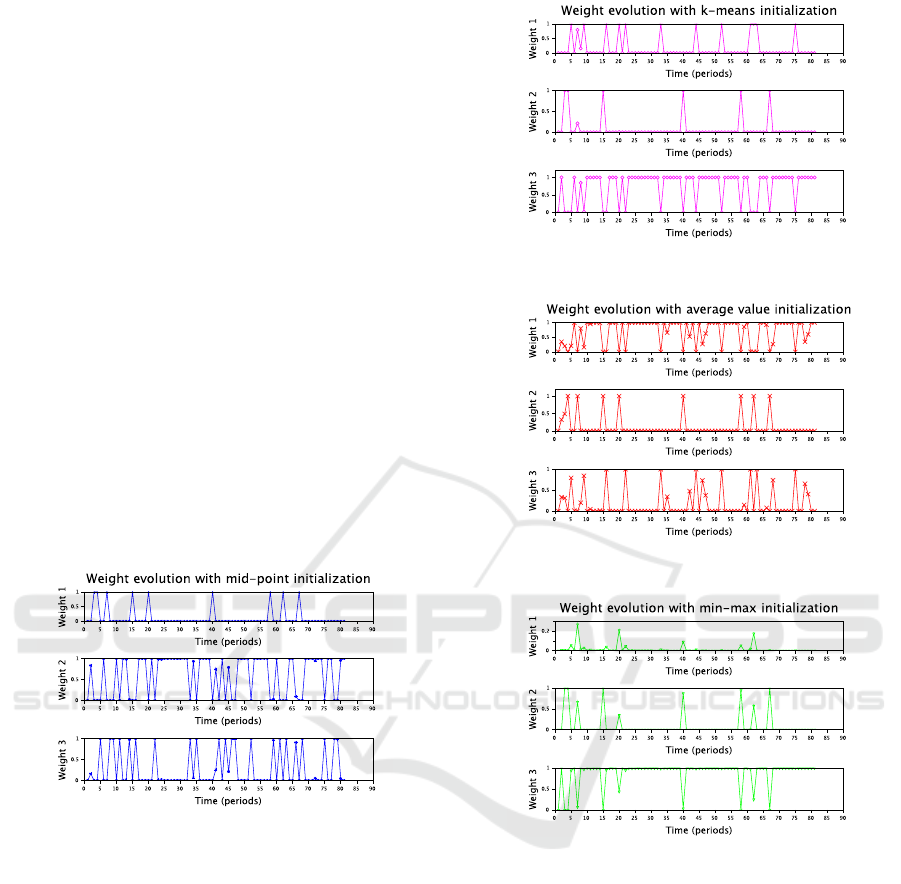
5.1 Evolution of Component Weights
A fragment of the evolution of the component
weights with the statistics initialized according to
Section 4.3.1 is demonstrated in Figure 3. It can be
seen that all three components are regularly active.
The plotted weights are approaching to 0 or 1 that
unambiguously expresses the activity of components.
The k-means based initial statistics give the similar
activity, see Figure 4. The initialization via methods
from Sections 4.3.3 is shown in Figure 5. It produces
a bit more probabilities close to 0.5. However, in gen-
eral, the result is similar to two first methods.
The last method based on minimum and maxi-
mum prior values according to Section 4.3.4 provides
only two detected components. Figure 6 shows at the
y-axis that the weights of the first component in the
top plot are too low, and this component is never de-
clared to be active.
Figure 3: Evolution of component weights with initial
statistics according to Section 4.3.1.
5.2 Evolution of Bounds
Comparing the evolution of the minimum and maxi-
mum bounds of individual entries within each compo-
nent, it can be noticed that a speed of localization of
stabilized estimate values is similar for the first three
methods, i.e., with exception of Section 4.3.4. The
bounds of one of the components are stabilized a bit
slower than the others: component 2 in the case of
Section 4.3.1, component 3 with Section 4.3.2 and
component 1 with Sections 4.3.3. The bounds of the
rest of the components detect their final values rela-
tively quickly. To save space, an example of the left
bound evolution is shown in Figure 7 for initialization
based on Section 4.3.1, where the difference between
the second component and the rest of them should be
Figure 4: Evolution of component weights with initializa-
tion according to Section 4.3.2.
Figure 5: Evolution of component weights with initializa-
tion according to Section 4.3.3.
Figure 6: Evolution of component weights with initializa-
tion according to Section 4.3.4.
noticed. The right bound evolution with the k-means
initialization due to Section 4.3.2 is demonstrated in
Figure 8, where the same can be said about the third
component.
Initialization according to Section 4.3.4 provides
a worse stabilization in search of stabilized values of
the bounds, see an example of the left bound evolu-
tion for the third component in Figure 9, where the
evolution of the left (minimum) bounds of individual
data entries is presented.
5.3 Clusters
Clusters of the most interesting pair of data entries
from the practical (hematological) point of view are
Initialization of Recursive Mixture-based Clustering with Uniform Components
455
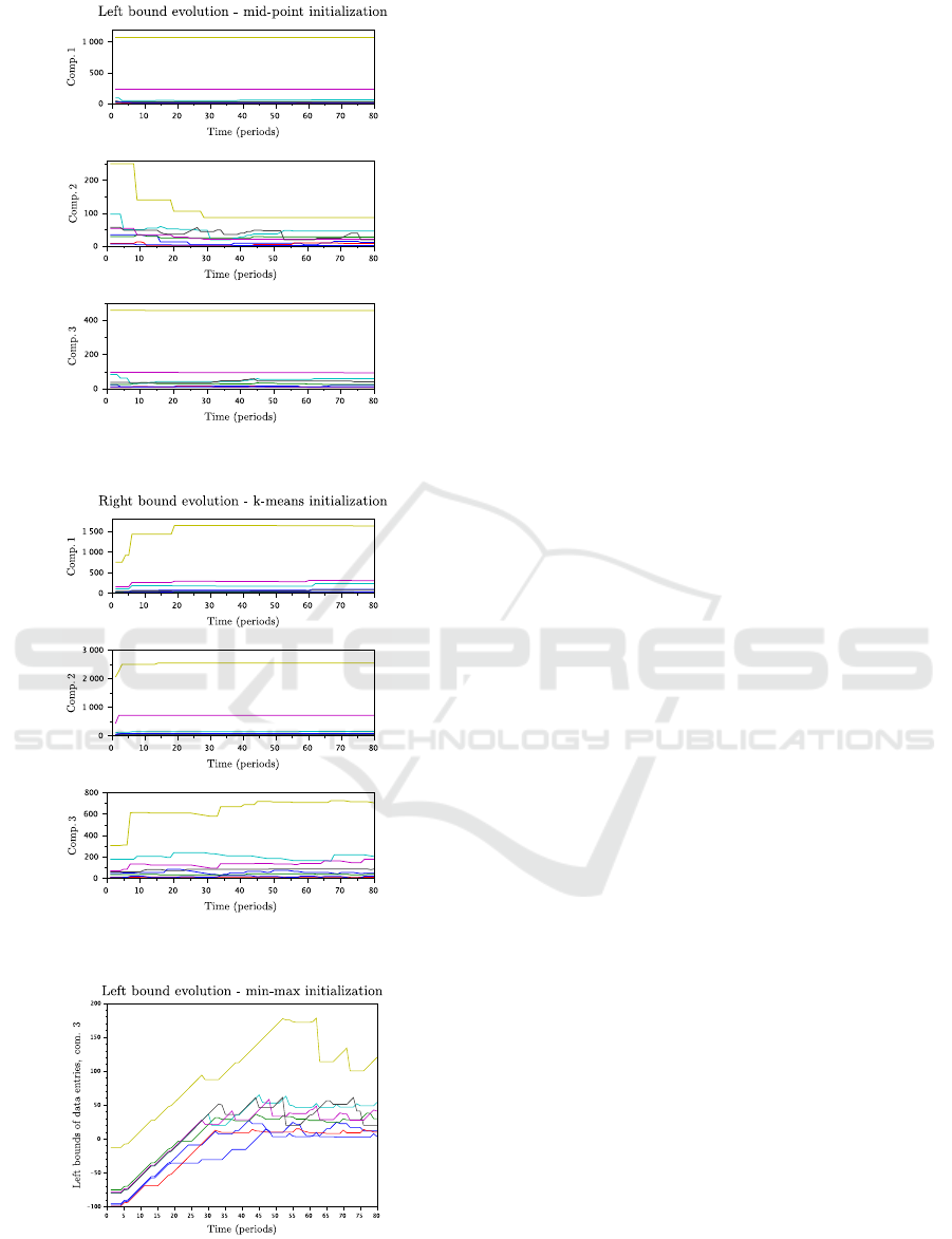
Figure 7: Evolution of the left bounds with initialization
according to Section 4.3.1.
Figure 8: Evolution of the right bounds with initialization
according to Section 4.3.2.
Figure 9: Evolution of the left bounds of the third compo-
nent with initialization according to Section 4.3.4.
presented here. The entries y
5;t
, which is the pre-
collection number of CD34+, and y
8;t
, which is the
concentration of CD34+/kg, are chosen. Their clus-
ters detected according to the estimated pointer value
can be seen in Figure 10, where comparison of results
initialized according to Sections 4.3.1, Section 4.3.2,
4.3.3 and 4.3.4 is demonstrated. The colors of the
clusters in the figure are chosen randomly in all of the
plots. The clusters are enumerated according to the
order in which they have been detected and plotted.
The shapes and the location of the detected clusters
should be compared.
The insignificant difference in the location of two
upper clusters can be seen in three first figures, while
in the bottom figure the clustering practically fails.
Only two data items are classified as belonging to the
first cluster, i.e., two clusters are detected.
For validation of clustering, the k-means algo-
rithm was run with whole data set. Results of this
clustering are given in Figure 11. It can be seen that
the shape and location of clusters are very similar in
Figure 11 and in the first and the third top plots in
Figure 10. The second top plot differs a bit.
5.4 Discussion
To summarize the experimental part of the work, it
can be stated that the obtained results of the recursive
clustering are validated by such the well-known the-
oretical counterpart as k-means. It should not be for-
gotten that k-means works with whole available data
set off-line, while the recursive clustering is based on
a completely different philosophy of on-line estima-
tion. The use of the normal approximation as the
proximity function for uniform components is also
successfully validated.
Among the discussed initialization techniques the
last method concerned with using the minimum and
maximum bound statistics has the worst results. This
indicates that the initialization via centers of uniform
components is a reasonable way of starting the esti-
mation algorithm. The initialization with randomly
chosen centers (which is not shown here to save
space) mostly leads to a dominance of one compo-
nents.
The described initialization still need an expert’s
intervention, namely, for a choice of the component
number. Surely, automatization of this process would
be preferable. This will be one of the tasks within the
current project.
ICINCO 2017 - 14th International Conference on Informatics in Control, Automation and Robotics
456
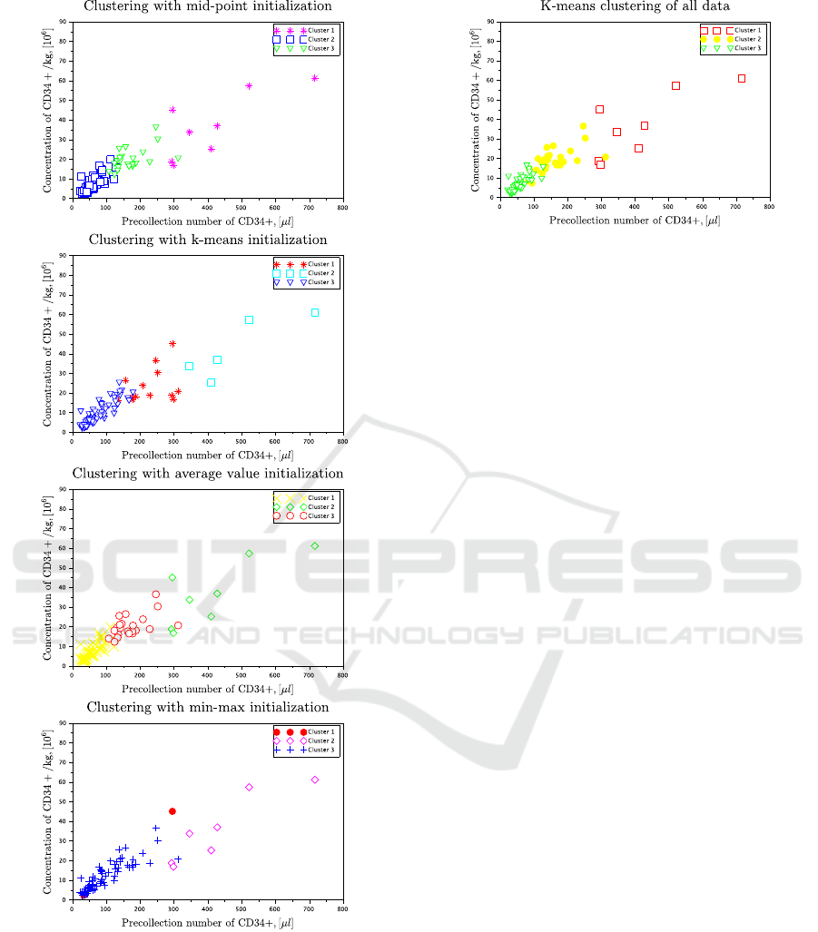
Figure 10: Comparison of clusters of y
5;t
and y
8;t
with
different initialization techniques obtained via recursive
mixture-based clustering.
6 CONCLUSIONS
The paper explores four approaches to a task of
initialization of recursive mixture-based clustering
with the uniform components under the Bayesian
Figure 11: Clusters of y
5;t
and y
8;t
detected by k-means.
methodology. The investigated approaches are based
on processing the prior data set with the aim of set-
ting the initial statistics of uniform components. The
comparison with the theoretical counterpart shows
that the presented results are promising.
However, there still exists a series of open prob-
lems in the discussed area, e.g., a start of forgetting
both the bounds (it must not be the same). Further,
modeling dependent uniformly distributed variables
with parallelogram-shaped clusters is still not solved.
This is also a subject of the planned research work.
ACKNOWLEDGEMENTS
The paper was supported by project GA
ˇ
CR GA15-
03564S.
REFERENCES
Roy, A., Pal, A., Garain, U. (2017). JCLMM: A Finite Mix-
ture Model for Clustering of Circular-Linear data and
its application to Psoriatic Plaque Segmentation, Pat-
tern Recognition, doi 10.1016/j.patcog.2016.12.016.
Hu, X., Munkin, M.K. and Trivedi, P.K., (2015). Estimating
Incentive and Selection Effects in the Medigap Insur-
ance Market: An Application with Dirichlet Process
Mixture Model. , Journal of Applied Econometrics,
30(7), p.1115-1143.
Bao, L. and Shen, X., (2016). Improved Gaussian mixture
model and application in speaker recognition. In 2nd
IEEE International Conference on Control, Automa-
tion and Robotics (ICCAR), p. 387–390.
Bouveyron, C., Brunet-Saumard, C. (2014). Model-based
clustering of high-dimensional data: A review. Com-
putational Statistics & Data Analysis. 71(0), p. 52–78.
Scrucca, L., (2016). Genetic algorithms for subset selection
in model-based clustering. Unsupervised Learning Al-
gorithms, p. 55–70, Springer International Publishing.
Fern
´
andez, D., Arnold, R., Pledger, S., (2016). Mixture-
based clustering for the ordered stereotype model.
Initialization of Recursive Mixture-based Clustering with Uniform Components
457

Computational Statistics & Data Analysis, 93, p.46–
75.
Browne, R.P. and McNicholas, P.D., (2015). A mixture of
generalized hyperbolic distributions. Canadian Jour-
nal of Statistics, 43(2), p.176–198.
Morris, K. and McNicholas, P.D., (2016). Clustering, clas-
sification, discriminant analysis, and dimension re-
duction via generalized hyperbolic mixtures. Compu-
tational Statistics & Data Analysis, 97, p.133–150.
Malsiner-Walli, G., Fr
¨
uhwirth-Schnatter, S., Gr
¨
un, B.,
(2016). Model-based clustering based on sparse finite
Gaussian mixtures. Statistics and computing, 26(1–2),
p.303–324.
Li, R., Wang, Z., Gu, C., Li, F., Wu, H., (2016). A novel
time-of-use tariff design based on Gaussian Mixture
Model. Applied Energy, 162, p.1530–1536.
O’Hagan, A., Murphy, T.B., Gormley, I.C., McNicholas,
P.D., Karlis, D., (2016). Clustering with the multi-
variate normal inverse Gaussian distribution. Compu-
tational Statistics & Data Analysis, 93, p.18–30.
Gupta, M. R. , Chen, Y. (2011). Theory and use of the EM
method. In: Foundations and Trends in Signal Pro-
cessing, vol. 4, 3, p. 223–296.
Scrucca, L. and Raftery, A.E., (2015). Improved initiali-
sation of model-based clustering using Gaussian hi-
erarchical partitions. Advances in data analysis and
classification, 9(4), p.447–460.
Melnykov, V., Melnykov, I. (2012). Initializing the EM al-
gorithm in Gaussian mixture models with an unknown
number of components, Computational Statistics &
Data Analysis, 56(6), p.1381–1395.
Kwedlo, W. (2013). A new method for random initializa-
tion of the EM algorithm for multivariate Gaussian
mixture learning, In: Proceedings of the 8th Inter-
national Conference on Computer Recognition Sys-
tems CORES 2013, (eds. R. Burduk, K. Jackowski,
M. Kurzynski, M. Wozniak, A. Zolnierek), Springer
International Publishing, Heidelberg, p. 81–90.
Shireman, E., Steinley, D. and Brusco, M.J., (2015). Exam-
ining the effect of initialization strategies on the per-
formance of Gaussian mixture modeling. Behavior
research methods, p.1–12.
Maitra, R., (2009). Initializing partition-optimization al-
gorithms. In: IEEE/ACM Transactions on Compu-
tational Biology and Bioinformatics (TCBB), 6(1),
p.144–157.
K
´
arn
´
y, M., Kadlec, J., Sutanto, E.L. (1998). Quasi-Bayes
estimation applied to normal mixture, In: Preprints
of the 3rd European IEEE Workshop on Computer-
Intensive Methods in Control and Data Processing
(eds. J. Roj
´
ı
ˇ
cek, M. Vale
ˇ
ckov
´
a, M. K
´
arn
´
y, K. War-
wick), CMP’98 /3./, Prague, CZ, p. 77–82.
Peterka, V. (1981). Bayesian system identification. In:
Trends and Progress in System Identification (ed. P.
Eykhoff), Oxford, Pergamon Press, 1981, p. 239–304.
K
´
arn
´
y, M., B
¨
ohm, J., Guy, T. V., Jirsa, L., Nagy, I., Ne-
doma, P., Tesa
ˇ
r, L. (2006). Optimized Bayesian Dy-
namic Advising: Theory and Algorithms, Springer-
Verlag London.
Nagy, I., Suzdaleva, E., K
´
arn
´
y, M., Mlyn
´
a
ˇ
rov
´
a, T. (2011).
Bayesian estimation of dynamic finite mixtures. Int.
Journal of Adaptive Control and Signal Processing,
vol. 25, 9, p. 765–787.
Suzdaleva, E., Nagy, I., Mlyn
´
a
ˇ
rov
´
a, T. (2015). Recursive
Estimation of Mixtures of Exponential and Normal
Distributions. In: Proceedings of the 8th IEEE In-
ternational Conference on Intelligent Data Acquisi-
tion and Advanced Computing Systems: Technology
and Applications, Warsaw, Poland, September 24–26,
p.137–142.
Casella, G., Berger R.L. (2001). Statistical Inference, 2nd
ed., Duxbury Press.
Nagy, I., Suzdaleva, E., Mlyn
´
a
ˇ
rov
´
a, T. (2016). Mixture-
based clustering non-gaussian data with fixed bounds.
In: Proceedings of the IEEE International conference
Intelligent systems IS’16, p. 265–271.
Suzdaleva, E., Nagy, I., Mlyn
´
a
ˇ
rov
´
a, T. (2016). Expert-based
initialization of recursive mixture estimation. In: Pro-
ceedings of the IEEE International conference Intelli-
gent systems IS’16, p. 308–315.
K
´
arn
´
y, M., Nedoma, P., Khailova, N., Pavelkov
´
a, L.,
(2003). Prior information in structure estimation. In:
IEE Proceedings, Control Theory and Applications,
150(6), pp. 643–653.
Nagy, I., Suzdaleva, E., Pecherkov
´
a, P. (2016). Compa-
rison of Various Definitions of Proximity in Mixture
Estimation. In: Proceedings of the 13th Interna-
tional Conference on Informatics in Control, Automa-
tion and Robotics (ICINCO), p. 527–534
Jain, A. K., (2010). Data clustering: 50 years beyond K-
means. Pattern Recognition Letters, 31(8), pp. 651–
666.
ICINCO 2017 - 14th International Conference on Informatics in Control, Automation and Robotics
458
