Learning from Simulated World - Surrogates Construction with Deep

Neural Network

Zong-De Jian

, Hung-Jui Chang

1,2

, Tsan-sheng Hsu

and Da-Wei Wang

Institute of Information Science, Academia Sinica, Taipei, Taiwan

Department of Computer Science and Information Engineering, National Taiwan University, Taipei, Taiwan

Keywords:

Deep Learning, Surrogate, Disease Simulator.

Abstract:

The deep learning approach has been applied to many domains with success. We use deep learning to construct

the surrogate function to speed up simulation based optimization in epidemiology. The simulator is an agent-

based stochastic model for inﬂuenza and the optimization problem is to ﬁnd vaccination strategy to minimize

the number of infected cases. The optimizer is a genetic algorithm and the ﬁtness function is the simulation

program. The simulation is the bottleneck of the optimization process. An attempt to use the surrogate function

with table lookup and interpolation was reported before. The preliminary results show that the surrogate

constructed by deep learning approach outperforms the interpolation based one, as long as similar cases of the

testing set have been available in the training set. The average of the absolute value of relative error is less

than 0.7 percent, which is quite close to the intrinsic limitation of the stochastic variation of the simulation

software 0.2 percent, and the rank coefﬁcients are all above 0.99 for cases we studied. The vaccination strategy

recommended is still to vaccine the school age children ﬁrst which is consistent with the previous studies. The

preliminary results are encouraging and it should be a worthy effort to use machine learning approach to

explore the vast parameter space of simulation models in epidemiology.

1 INTRODUCTION

Simulation models are built so that we can experiment

with them to gain insight about subjects investigated.

With the current success of machine learning, espe-

cially deep learning, it is worth exploring about using

machine learning technique to learn from the simula-

tion models. We explore the possibility by using the

deep neural network to construct a surrogate function

as the cost function instead of running real simulation

when applying the genetic algorithm to search for ef-

fective vaccination strategy in the domain of public

health.

Agent-based stochastic simulations have been ap-

plied widely for the study of infectious diseases (Ger-

mann et al., 2006)(Chao et al., 2010). Comparing to

the mathematical models, the ﬂexibility to easily in-

corporate detailed disease control strategies into sim-

ulation model is one of its strength. However, it still

needs a signiﬁcant amount of computing resources.

Epidemiologists usually have to carefully craft the

scenarios to demonstrate their points. Vaccination

can effectively mitigate the impact of the pandemic

ﬂu with an appropriate vaccinating strategy which

might depend on an amount of available vaccines. In-

stead of comparing a few strategies selected by do-

main experts, we formulate it as an optimization prob-

lem and employ genetic algorithms to search for the

best vaccination priority. The search space can po-

tentially contain many dimensions, for example, the

house-hold structure is one of the important dimen-

sions (Chang et al., 2015). In this paper, we focus on

the dimension of vaccination allocation.

The supply of the vaccine is usually limited, the

disease control agency has to decide the amount of

vaccine allocated to various groups. Without a doubt,

the health care professionals should get the highest

priority. Then the agency determined how much to

distribute to different age groups. How to determine

the number of doses to each age group is an impor-

tant issue. The objective can also be complicated, for

example, one can search for a strategy to minimize

economic impact, or to minimize the total number of

infected cases. In this paper, the goal is to minimize

the total number of infected cases.

For a given scenario, that is the setting of our sim-

ulation module, the gene encodes the vaccine distribu-

tion among age groups and the ﬁtness function is the

Jian, Z-D., Chang, H-J., Hsu, T-s. and Wang, D-W.

Learning from Simulated World - Surrogates Construction with Deep Neural Network.

DOI: 10.5220/0006418100830092

In Proceedings of the 7th International Conference on Simulation and Modeling Methodologies, Technologies and Applications (SIMULTECH 2017), pages 83-92

ISBN: 978-989-758-265-3

total number of infected cases. The ﬁtness evaluation

is done by running the simulation module.

Each simulation run takes about 3 minutes, thus

the ﬁtness evaluation becomes the bottleneck of the

optimization process. Using a faster approximation

in place of the true ﬁtness function, in our case the

simulation program, is called surrogated-assisted evo-

lutionary computation (Jin, 2011). The idea was ﬁrst

suggested in the mid-1980s (J.J. Grefenstette, 1985).

A surrogate function combines table lookups and lin-

ear interpolation was suggested in (Jian et al., 2016).

In this study, we use the deep neural network to con-

struct the surrogate function and compare it with the

previous interpolation based one.

The accuracy is measured by the relative error,

that is the difference between the output of surrogate

function and the simulation divided by the output of

the simulation. The average of the absolute value

of the relative errors of the surrogate functions con-

structed by the deep neural network approach range

from 0.18 percent to 0.68 percent for different train-

ing sets and testing sets. When the training sets have

cases similar to the testing sets, the surrogate con-

structed by deep neural network usually performs bet-

ter than the interpolation based one. The search re-

sults with the surrogate in place of the simulation sys-

tem have error margin less than one percent. The

rank correlation coefﬁcients of the surrogates are bet-

ter than 99 percent.

2 MATERIAL AND METHOD

Our approach to search for the optimal vaccina-

tion strategy belongs to the general category of

simulation-based optimization (Gosavi, 2015). We

ﬁrst introduce our simulation software, followed by

a description of our optimization procedure.

We use the simulation software developed in our

laboratory (Tsai et al., 2010). Below is a brief de-

scription of how the simulation works. It is a stochas-

tic discrete time agent-based model. The mock pop-

ulation of the model is constructed according to na-

tional demographics from Taiwan Census 2000 data

(http://eng.stat.gov.tw/). The connection between any

two individuals indicates the possibility of daily and

relatively close contact which could result in a suc-

cessful transmission of the ﬂu virus. An important

virus-dependent parameter is the transmission proba-

bility, denoted by p

trans

. It is the probability that an

effective contact results in an infection. An individ-

ual can be in one of the following four states, suscep-

tible(S), exposed(E), infectious(I), and recovered(R).

when an effective contact happens between an indi-

vidual in the state S and an individual in the state I,

the susceptible individual will become exposed with

probability p

trans

. According to the disease natural

history, an exposed individual becomes infectious and

an infectious individual becomes recovered, in our

setting the average incubation period is 1.9 days and

the average infectious period is 4.1 days (Germann

et al., 2006). A contact group is a daily close associ-

ation of individuals, where every member has a con-

tact probability to have effective contact with all other

members in the same group. There are eleven such

contact groups in the model, they are communities,

neighborhood, household cluster, household, work-

group, high school, middle school, elementary school,

daycare center, kindergarten, and playgroup (Chang

et al., 2015). The population size of Taiwan is about

22.12 million. There are about 1.72 million

preschool

children

(0-5 years old), about 2.36 million

elemen-

tary school children

(6-12 years old), about 0.99 mil-

lion

middle school children

(13-15 years old), about

0.97 million

high school children

(16-18 years old),

about 3.86 million

young adults

(19-29 years old),

about 10.28 million

adults

(30-64 years old), and

about 1.94 million

elders

(65+ years old).

Each individual can belong to several contact

groups simultaneously at any time. The duration of

a simulation run is set at 365 days. Each day has

two 12-hour periods, daytime and nighttime respec-

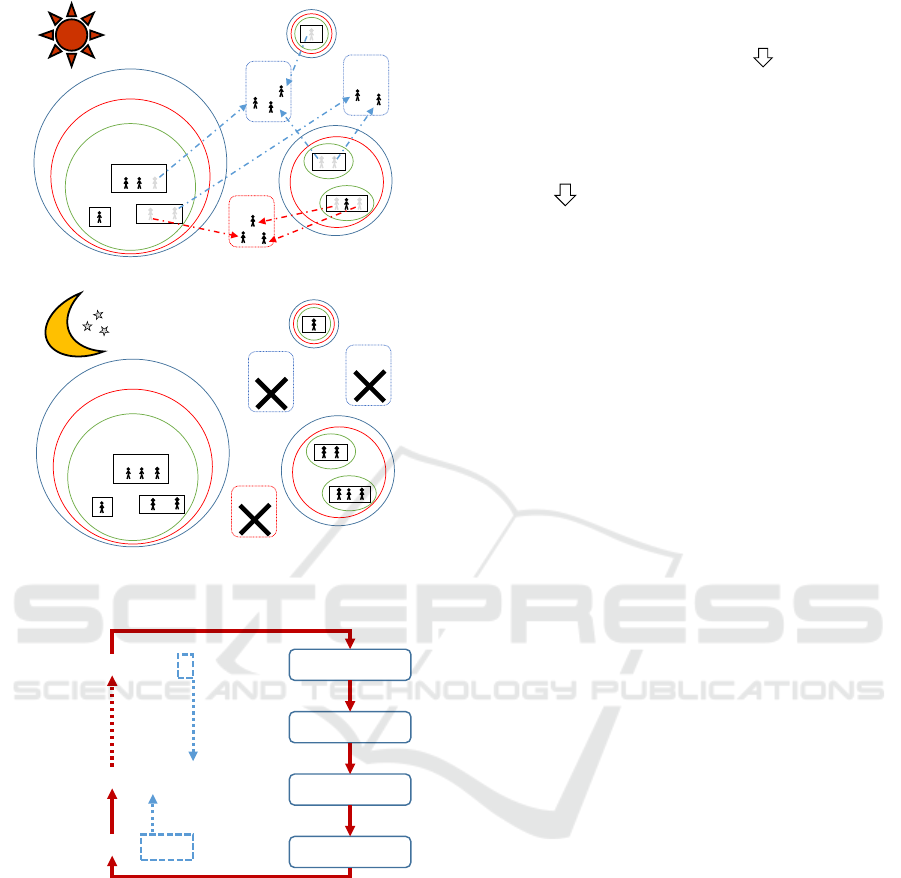
tively. Behaviors of individuals are depicted in Fig-

ure 1. During daytime, contact occurs in all contact

group. School aged children go to schools. There

are around 7.8% school aged children do not go to

school in Taiwan. They stay home in our simulation.

Preschool children go to a daycare center, kinder-

garten or playgroup. Young adults and adults go to

workgroup. In the nighttime, contact occurs only in

communities, neighborhoods,household clusters, and

household.

The model parameters are similar to ones in a

study by (Germann et al., 2006), with modiﬁcations to

ﬁt Taiwan situation better with the help of study out-

come in contact diary study (Fu et al., 2012). We re-

call that the stochastic variation of the simulation sys-

tem is reported to be around 0.2 percent (Tsai et al.,

2010).

In this paper, our setting is similar to our previous

study about surrogates functions(Jian et al., 2016):the

rans is set at 0.1, the vaccine is available 30 days af-

ter the index case occurred, total 2.5 million of doses

are applied to different age groups according to the

priority.. However, we only focus on the case that the

vaccine efﬁcacy,VEi and VEs, are ﬁxed at 0.9 (Basta

et al., 2008). The vaccine is available 30 days after

the index case occurred, total available vaccine are all

SIMULTECH 2017 - 7th International Conference on Simulation and Modeling Methodologies, Technologies and Applications

Community

Working

group

School

neighborhood

Household cluster

Household

Working

group

(a) Contact behavior in daytime.

Community

Working

group

School

neighborhood

Household cluster

Household

Working

group

(b) Contact behavior in nighttime.

Figure 1: Contact behavior.

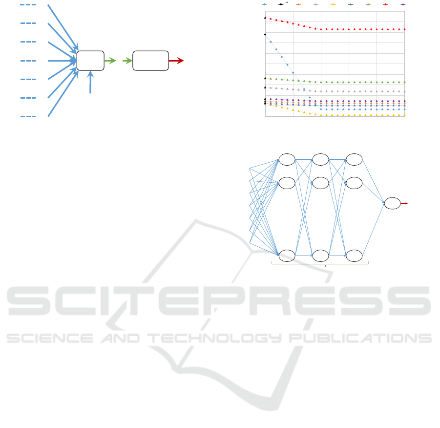
Simulated annealing

Selection

Crossover

Mutation

ܲܽݎ݁݊ݐݏ

௜

= { Ƹ݌, Ƹ݌, … , Ƹ݌ }

ܲܽݎ݁݊ݐݏ

௜ାଵ

= { Ƹ݌, Ƹ݌, … , Ƹ݌}

ܥ݄݈݅݀ݎ݁݊

௜

= { Ƹ݌, Ƹ݌, … , Ƹ݌ }

Copy the best Ƹ݌

Copy the first nine Ƹ݌

Check the

stopping criteria

Figure 2: Process of HSAGA.

administered to individuals.

A vaccination priority is denoted by p =

,...,x

), where x

is the amount of vaccine for

the age group i and it is less than the population of age

group i. We use p

to denote vectors with only those

value of x

are nonzero and α is a set with numberings

of each age group. For example p

2,3

denote the set

of vaccination priority with non-zero entries for age

group 2 and age group 3 and p

i, j,k

to denote the set of

vectors with 3 non-zero entries. Let p =

0 denote the

baseline case with no vaccination. We use Sim(p) to

denote the number of infected cases reported by the

simulation program with vaccination priority p.

Ƹ݌

஺

= ( 30, 70, 91, 103, 205, 240, 250 )

Ƹ݌

஻

= ( 10, 20,

40, 77, 121, 210, 250 )

Ƹ݌

஺

ᇲ

= ( 30,

40, 77, 121, 205, 240, 250 )

Ƹ݌

஻

ᇲ

= ( 10, 20,

70, 91, 103, 210, 250 )

Random select two numbers: [ ૜૞, ૚૞૙]

Figure 3: Crossover of HSAGA.

Ƹ݌ = ( 3, 25, 70, 90, 150, 200, 250 )

Random select a index, change a random number [83],

and re-sort the chromosome.

Ƹ݌’ = ( 3, 25, 70, 83, 90, 200, 250 )

Figure 4: Mutation of HSAGA.

We use the genetic algorithm to search for the

optimal vaccine strategy. A simulated annealing

step is introduced to speedup the process. In

the hybrid simulated annealing genetic algorithm

(HSAGA), the population is consists of vaccine al-

locations represented in preﬁx sum format. That

is p = (20, 50,50, 70,20, 30,10) can be rewritten as

ˆp = (20, 70,120,190, 210,240,250), since the total

amount of vaccine is always 2.5 millions the last co-

ordinate can be dropped. The population size is ten,

and each iteration begins with simulated annealing

step to perturb each candidate, followed by the se-

lection, crossover, and mutation steps. Figure 2 is the

ﬂow-chart of the process. For a given allocation, we

carried out 5 simulation runs, and the ﬁtness score is

the average of the values of the objective function of

each run. The best solution of the previous generation

and the ﬁrst nine solutions for this generation become

the candidates of next generation. At the beginning

of each iteration, we carry out a simulated annealing

step for each candidate. It is a temperature controlled

mutation, i.e., we mutate each candidate according to

the temperature (that is the number of iterations up to

the point in our case). The process stops at 200 itera-

tions and the early stop condition is that ﬁve consec-

utive iterations consist of the same candidates. Given

two genes (vaccine priorities), the crossover operation

is the following: Randomly generate a pair of num-

bers g

where 0 ≤ g

≤ g

≤ 250, if the interval

] covers the same number of chromosomes in

both genes, then we exchange the covered part. The

segment of chromosomes x

is covered by interval

] if and only if x

i−1

≤ g

≤ x

and x

≤ g

≤

j+1

. Figure 3 is an example of the crossover oper-

ation. We randomly increase g

or decrease g

if a

direct exchange is invalid, that is the length of cov-

ered segments differ. A more detailed description can

be found in (Jian et al., 2016).

The mutation operation is deﬁned as following:

Randomly pick index i and randomly generate a num-

ber x, replace x

with x and sort the resultant sequence.

Figure 4 is an illustration of the mutation operation.

Learning from Simulated World - Surrogates Construction with Deep Neural Network

ଵ

ଶ

ଷ

ସ

ହ

଺

଻

Sum Function

ଶ

ଷ

ସ

ହ

଺

଻

ଵ

ݖ ݂(ݖ)

Figure 5: The model of Sur

(p).

2.1 Surrogates with Deep Learning

Deep learning gained a lot of attention with a few

highly publicized success. It is a branch of machine

learning, and one of its basic ingredients is the ar-

tiﬁcial neural network. The word deep referring to

the fact that the model is built with multilayer per-

ceptrons(MLP). Each perceptron has a transformation

function to produce output to next perceptrons with

the inputs from connected perceptrons at the previous

stage. During the training phase, the prediction er-

ror is determined by the loss function, and the error

triggering a weight adjustment procedure, backprop-

agation is the most commonly applied method.

In our research, we use deep neuron networks

(DNN) as the model of the surrogate function. In

this study, we use Keras on Theano running on Nvidia

GeForce GTX 1080 Graphics Card (Keras, 2015).

The surrogate function takes the vaccine alloca-

tion of seven age groups, p, as the input and the output

is the total number of infected cases.

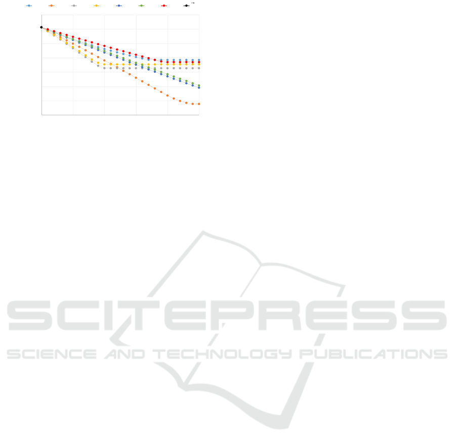
We ﬁrst applied single perceptron model with the

linear function to check if there exist good linear sur-

rogates. The single perceptron model is shown in Fig-

ure 5, in which w

denotes the weight, and b is the

bias. We let the activation function to be a linear func-

tion, i.e., f(z) = z and the output of the single percep-

tron model is denoted by Sur

Sur

(p) = f(z) = z =

∑

i=1

) + b (1)

As shown in Figure 6, the slope approaching zero

when the vaccine allocation is approaching the size

of the population of that age group. As expected, we

can see that the number of infected cases of other age

groups is also affected by the amount allocated to one

speciﬁc age group.

We next move on to the deep neural network

with nonlinear activation function. The architecture

is shown in Figure 7. The output of the deep neural

500,000

1,000,000

1,500,000

2,000,000

2,500,000

3,000,000

3,500,000

4,000,000

7,000,000

7,200,000

7,400,000

7,600,000

7,800,000

8,000,000

8,200,000

8,400,000

8,600,000

8,800,000

9,000,000

0 500,000 1,000,000 1,500,000 2,000,000 2,500,000

cases for each age group

total cases

doses

t 0 1 2 3 4 5 6 7

ଷ

ଵ

௣

య

ଶ

௣

య

ଷ

௣

య

ସ

௣

య

ହ

௣

య

଺

௣

య

଻

௣

య

Figure 6: Sim(p

) with p

∈ P

ଵ

ଶ

ଷ

ସ

ହ

଺

଻

ଵ

ଶ

ଵ

ଵଶ଻

ଵ

. . . . . .

ଵ

ଶ

ଵଶ଻

ଶ

. . . . . .

ଵ

ଷ

ଶ

ଷ

ଵଶ଻

ଷ

. . . . . .

ଵ

ସ

ܵݑݎ

ଶ

஽

(݌)

Hidden layers Output layerInput layer

Figure 7: The model of Sur

(p).

network is denoted by Sur

(p). It is a fully connected

architecture, that is the outputs of every neuron in this

layer are inputs for every neuron in next layer. We add

three hidden layers, and each layer has

∑

i=1

= 127

perceptrons, which corresponding to the number of

all the combinations of the seven age groups. The ac-

tivation function is exponential linear units (ELUs),

it can handle non-linear relations and outperform the

traditional rectiﬁed linear unit(ReLU)(Clevert et al.,

2015).

2.2 Surrogates with Interpolation

We compare the surrogates learnt by neural networks

with the interpolation based ones we constructed be-

fore. We ﬁrst give a brief description of the previ-

ous work, and the details can be found in (Jian et al.,

2016).

To apply interpolation, we need a set of reference

points, denoted by P

, the values of these points are

the simulation results. In other words, points in p

are

entries of the lookup table. If p ∈ P

the result, Sim(p),

is the total number of infected cases by simulation. If

p /∈ P

, then Sim(p) denote the estimated total number

of infected cases by interpolation. We ﬁrst sampled

26 points for each age group, there are 182 points in

total. The 26 points are evenly spaced up to 2.5 mil-

SIMULTECH 2017 - 7th International Conference on Simulation and Modeling Methodologies, Technologies and Applications

5,500,000

6,000,000

6,500,000

7,000,000

7,500,000

8,000,000

8,500,000

9,000,000

0 500,000 1,000,000 1,500,000 2,000,000 2,500,000

total cases

doses

p1 p2 p3 p4 p5 p6 p7 0

ଵ

ଶ

ଷ

ସ

ହ

଺

଻

Figure 8: Sim(p

) with p

∈ P

lion doses of vaccine. Figure 8 shows the value of

each point. We then deﬁne the effect of introducing

strategy p

, denoted by ∆(p

) as following:

∆(p

) = Sim(p

) − Sim(

0) (2)

To approximate the effect of a point p, we add the

effect of each component and denote it by Sur

(p):

Sur

(p) = Sim(

0) +

∑

i=1

∆(p

) (3)

If the value of p

is not sampled, the linear interpo-

lation is applied to estimate ∆(p

). As expected, this

simple surrogate does not capture the interaction be-

tween age groups well. We build a lookup table with

entries in the form of p

i, j

to capture the interactions

between age groups. For each age group i, ﬁve evenly

spaced values are determined. Given two age groups,

we take one value from each group to form a vacci-

nation strategy and carry out the simulation. There

are total 21× 5 × 5 = 525 such points. For a point

p = (x

,...,x

), we slightly abuse the notation and

use p

j,k

denote the point with the same value as p

in j

and k

dimensions and all other dimensions are

zero. The adjustment term for the interaction between

dimension j and k, denoted by δ(p

j,k

), is deﬁned as

following:

δ(p

j,k

) = Sim(p

j,k

) − Sur

j,k

) (4)

When p

j,k

is not sampled, a bilinear interpolation

is applied. The surrogate with the two age group in-

teraction adjustment, denoted by Sur

(p), is deﬁned

as following:

Sur

(p) = Sim(

0)+

∑

i=1

∆(p

) +

∑

j=1

∑

k= j+1

δ(p

j,k

) (5)

3 RESULTS

We collected two sets of points in our previous study.

First, the set of base points, p

, which are the points

serve as the sampled points while developing interpo-

lation based surrogate. Second, the set of points eval-

uated during the execution of HSAGA and we denote

the set by P

. For this study, we further evaluate a

set of points, denoted by P

, which are points have

3 age groups assigned none zero entries. There are

= 36 combinations and for each dimension, we

evenly sampled 4 points up to the population size of

that age group. In other words, the increment is 1/4

of the size of the age group. We also limit the total

amount is no more than 4 million doses and each age

group gets at most 2.5 million. We note that because

of the choice of increment P

0. There size of

is 707, P

is 988, and P

is 1557. Our training and

testing data are drawn from these three sets. We set

epoch to be 10 thousand, mini-batch to be 10 and we

use mean absolute error (MAE) as our loss function

and Nadam as optimizer (Dozat, 2015).

We compare surrogates learnt by DNN with inter-

polation based surrogates. There are several settings.

We always use D

to denote the training set and D

to denote the testing set. The interpolation based sur-

rogate does not have the training phase, only testing

set matters for their evaluation. We use the relative er-

ror between the output of surrogate and the simulation

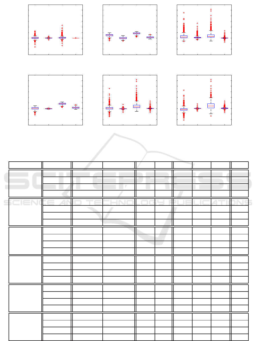
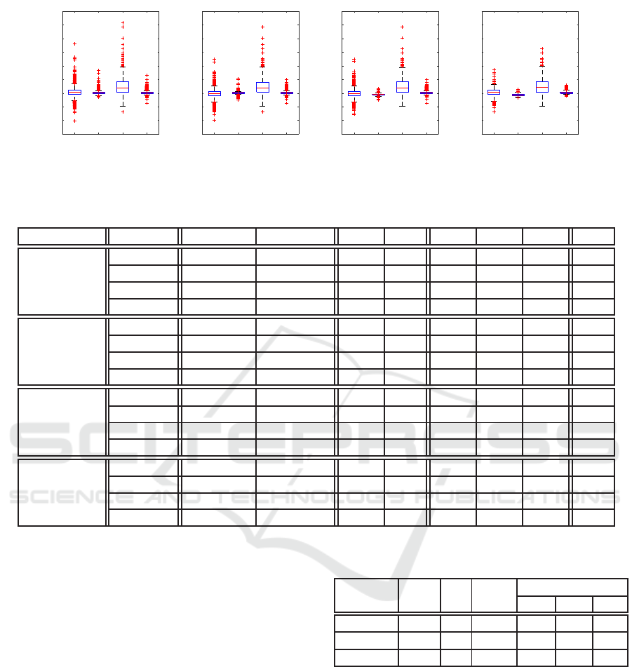
result and use box plot to visualize the results.

In Figure 9(a), there is no error for Sur

(p) be-

cause the testing data is P

which are the reference

base for interpolation. Similarly, the error for Sur

(p)

is from points with pattern p

j,k

. From the fact that

Sur

(p) is the result of a thorough training phase and

that it has much larger error comparing with Sur

(p),

it is safe to say that the relation between vaccine allo-

cation and the total number of infected case reduced

is not a simple linear one.

In Figure 9(b), we note that P

contains points

with many non-zero dimensions because the ge-

netic algorithm starts with random points and grad-

ually converge to points concentrating on vaccinat-

ing school children. We can see that Sur

(p) and

Sur

(p) obviously over-estimate the value, although

the spreading patterns are more or less similar in all

four cases.

In Figure 9(c), the testing data P

contains points

with 3 non-zero entries. Compared with Figure 9(a)

the over-estimating phenomenon is even more obvi-

ous, even Sur

(p) can not remedy the fact that the

interaction among three age groups is not captured.

We can see that Sur

(p) is outperformed by

Sur

(P) in Figure 9(a) and 9(c) . The reason is that

Learning from Simulated World - Surrogates Construction with Deep Neural Network

Sur

(p) Sur

(p)

-15

-10

-5

Relative Error (%)

(a) D

= P

, D

= P

Sur

(p) Sur

(p)

-15

-10

-5

Relative Error (%)

(b) D

= P

, D

= P

Sur

(p) Sur

(p)

-15

-10

-5

Relative Error (%)

= P

, D

= P

Sur

(p) Sur

(p)

-15

-10

-5

Relative Error (%)

(d) D

= P

, D

= P

Sur

(p) Sur

(p)

-15

-10

-5

Relative Error (%)

(e) D

= P

, D

= P

Sur

(p) Sur

(p)

-15

-10

-5

Relative Error (%)

(f) D

= D

= P

Figure 9: Box plot with different surrogates.

Table 1: Detail data of Figure 9.

surrogate avg of abs max of abs avg SD Q

IQR

Figure 9(a)

Sur

(p) 0.80 8.00 0.11 1.25 -0.38 0.09 0.57 0.95

Sur

(p) 0.23 1.71 0.05 0.31 -0.14 0.08 0.21 0.34

Sur

(p) 0.77 11.32 0.48 1.43 0.00 0.08 0.70 0.70

Sur

(p) 0.00 0.04 0.00 0.00 0.00 0.00 0.00 0.00

Figure 9(b)

Sur

(p) 2.65 4.69 2.61 1.06 2.04 2.82 3.35 1.30

Sur

(p) 0.68 2.79 0.01 0.88 -0.52 -0.01 0.60 1.11

Sur

(p) 4.16 5.87 4.16 0.84 3.62 4.23 4.75 1.13

Sur

(p) 0.86 3.28 0.80 0.83 0.20 0.58 1.29 1.09

Figure 9(c)

Sur

(p) 1.76 22.77 1.43 2.28 0.15 0.96 2.11 1.96

Sur

(p) 0.66 13.30 0.56 1.00 0.09 0.36 0.73 0.64

Sur

(p) 2.42 25.77 2.23 2.84 0.54 1.52 3.04 2.50

Sur

(p) 0.22 6.48 0.15 0.44 -0.01 0.08 0.19 0.20

Figure 9(d)

Sur

(p) 1.00 5.81 0.02 1.30 -0.66 0.17 0.97 1.63

Sur

(p) 0.19 0.73 -0.14 0.19 -0.27 -0.14 -0.02 0.25

Sur

(p) 4.16 5.87 4.16 0.84 3.62 4.23 4.75 1.13

Sur

(p) 0.86 3.28 0.80 0.83 0.20 0.58 1.29 1.09

Figure 9(e)

Sur

(p) 1.20 17.81 0.21 1.85 -0.62 0.13 0.88 1.50

Sur

(p) 0.29 3.56 -0.24 0.30 -0.37 -0.24 -0.11 0.26

Sur

(p) 2.42 25.77 2.23 2.84 0.54 1.52 3.04 2.50

Sur

(p) 0.22 6.48 0.15 0.44 -0.01 0.08 0.19 0.20

Figure 9(f)

Sur

(p) 1.30 16.21 -0.85 1.60 -1.58 -0.77 -0.04 1.54

Sur

(p) 0.18 3.88 -0.10 0.25 -0.21 -0.08 0.04 0.24

Sur

(p) 2.59 25.77 2.44 2.50 0.44 2.09 4.15 3.72

Sur

(p) 0.37 6.48 0.31 0.64 0.00 0.07 0.38 0.38

the training data and testing data are in a different cat-

egory and Sur

(P) is designed to work with those spe-

cial categories well. In Figure 9(b) the testing set con-

tains more randomly sampled data, we see Sur

(p)

SIMULTECH 2017 - 7th International Conference on Simulation and Modeling Methodologies, Technologies and Applications

Sur

(p) S ur

(p) Sur

(p)

-15

-10

-5

Relative Error (%)

(a) 20%, 80%

Sur

(p) S ur

(p) Sur

(p)

-15

-10

-5

Relative Error (%)

(b) 40%, 60%

Sur

(p) S ur

(p) Sur

(p)

-15

-10

-5

Relative Error (%)

Sur

(p) S ur

(p) Sur

(p)

-15

-10

-5

Relative Error (%)

(d) 80%, 20%

Figure 10: Box plot which cutting sample data P

by different percentage for D

and D

Table 2: Detail data of Figure 10.

surrogate avg of abs max of abs avg SD Q

IQR

Figure 10(a)

Sur

(p) 1.14 18.00 0.30 1.64 -0.46 0.30 1.10 1.57

Sur

(p) 0.30 8.29 0.09 0.49 -0.18 0.04 0.82 0.46

Sur

(p) 2.60 25.77 2.45 2.55 0.43 2.05 4.15 3.72

Sur

(p) 0.38 6.48 0.32 0.65 0.00 0.07 0.39 0.39

Figure 10(b)

Sur

(p) 1.06 12.48 -0.21 1.57 -0.92 -0.15 0.59 1.51

Sur

(p) 0.26 5.20 0.12 0.39 -0.02 0.14 0.30 0.32

Sur

(p) 2.54 24.22 2.39 2.49 0.39 1.99 4.11 3.72

Sur

(p) 0.38 5.07 0.32 0.65 0.00 0.06 0.38 0.38

Figure 10(c)

Sur

(p) 1.08 12.44 -0.22 1.60 -0.93 -0.18 0.57 1.50

Sur

(p) 0.44 2.40 -0.43 0.27 -0.57 -0.42 -0.27 0.30

Sur

(p) 2.62 24.22 2.47 2.58 0.46 2.01 4.18 3.72

Sur

(p) 0.39 5.07 0.33 0.66 0.00 0.07 0.40 0.40

Figure 10(d)

Sur

(p) 1.13 8.51 0.24 1.55 -0.50 0.30 1.07 1.57

Sur

(p) 0.59 1.73 -0.57 0.33 -0.81 -0.58 -0.35 0.46

Sur

(p) 2.70 16.24 2.55 2.53 0.47 2.14 4.31 3.84

Sur

(p) 0.38 3.00 0.33 0.61 0.00 0.08 0.44 0.44

performs better. In the next few experiments, we al-

low training set to contain the testing set. We are fully

aware that training set and testing set should be dis-

joint in general. But here we want to demonstrate

the advantage of the machine learning approach, that

is by providing proper training set the performance

can be enhanced greatly. As expected, in Figure 9(d)

and Figure 9(f) we can see Sur

(p) learned a better

approximation function and outperforms Sur

(p). In

Figure 9(e), Sur

(p) performs better and we suspect

that the testing set, points with three non-zero ele-

ments, is very close to the table lookup entries, points

with two non-zero elements. And this particular phe-

nomenon deserve further investigation.

A proper evaluation should have the disjoint train-

ing set and testing set. We take the union of P

, P

and

as the sample set. And then partition the whole

set into training and testing set. The result is shown

in Figure 10, the percentage on the left is the portion

of the training set and left is the testing set. Observ-

ing the quartile,Q

andQ

, of Sur

(p) and Sur

(p),

Table 3: The best allocation of HSAGA with each ﬁtness

function.

F C I N

p (×10

doses)

ES MS HS

Sim(p) 4.99 72 988 97 79 74

Sur

(p) 4.98 75 1020 100 81 69

Sur

(p) 4.99 87 1135 96 78 76

’ F ’: ﬁtness function

’ C ’: total cases (×10

)

’ I ’: total iterations

’ N ’: total allocations

’ ES ’:

elementary school children

’ MS ’:

middle school children

’ HS ’:

high school children

we can see the effect of learning. Also, the width of

the spreading pattern decreases as the training data in-

creases. We include all the numerical data for the plot

in Table 2. There are two columns ”avg” and ”avg

of abs”, the former is the average of the relative error

and the latter is the average of the absolute value of

Learning from Simulated World - Surrogates Construction with Deep Neural Network

relative error.

We then put Sur

(p) to the application test, and

use it as the ﬁtness function in HSAGA to search for

the appropriate vaccine strategy. The training set for

the function is P

. The result is shown in

Table 3. Three methods produce similar results and

the conclusion conﬁrms to previously reported stud-

ies: that the best strategy is to vaccinate school chil-

dren.

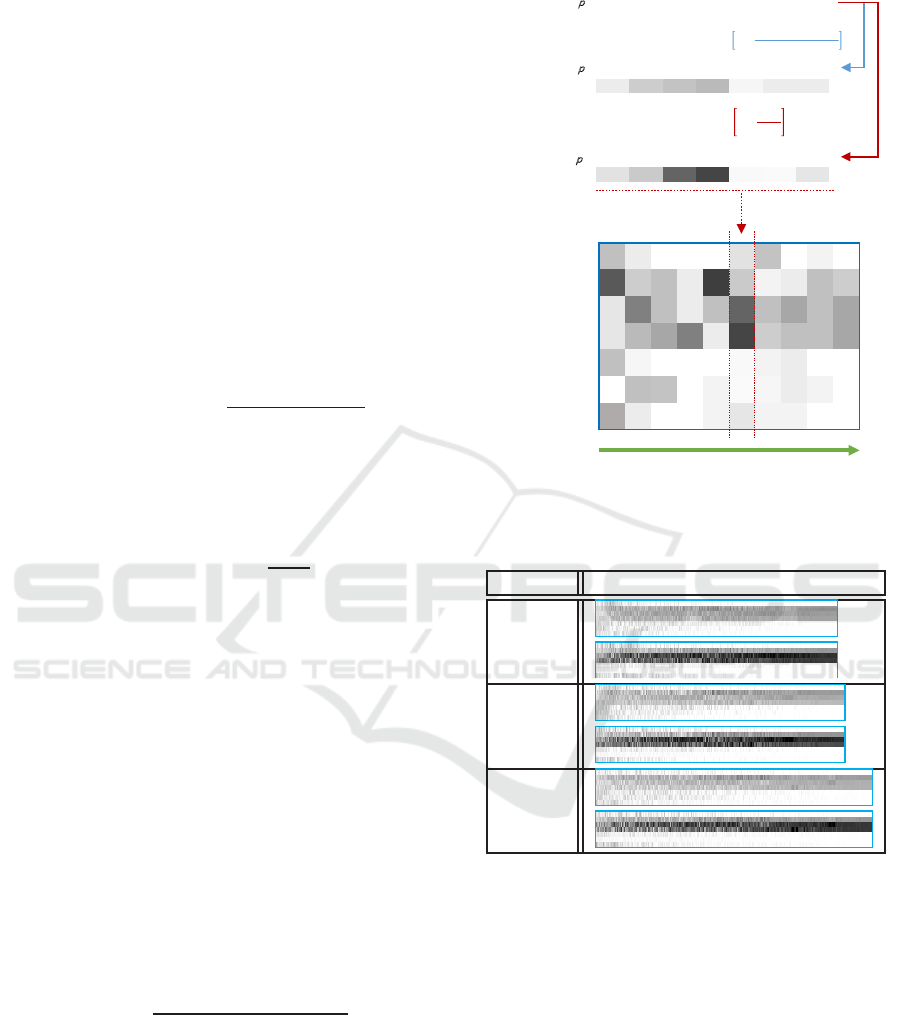
To visualize the vaccine allocations and to facil-

itate further exploration, a method to encode the al-

location by gray level was developed in (Jian et al.,

2016). We brieﬂy recap the method. There are two

encoding schemes,volume scheme and ratio scheme.

For volume scheme, the color white is to denote zero

doses and black for 2.5 million doses. Let x

be the

number of doses for age group i, the gray level is com-

puted by the following equation:

volume

= 255× [1−

2.5 million doses

] (6)

For the ratio scheme, the color white to denote

zero percent of the age group i vaccinated and black

hundred percent and we used #AG

to denote the pop-

ulation of age group i. The gray level is computed by

following equation:

ratio

= 255× [1 −

#AG

] (7)

After each age group is assigned a gray level accord-

ing to the equation above, we use a line segment with

that gray level to represent vaccination level of each

age group, as shown in the top half of Figure 11. The

allocation is then represented by stacking the seven

line segment vertically (in the middle part of Figure

11, we put the line segment horizontally).

For a set of ordered allocations, the line segment

for each allocation is stitched together according to

the ordering. The sequence of allocations is sorted

from left to right where the better allocations are on

the right hand side. As shown in Table 4, the visual

effect of concentration on school children is obvious.

For genetic algorithms, the rank preserving sur-

rogates are preferred. One metric to measure the ﬁ-

delity of surrogates is rank correlation coefﬁcient (r

)

(Loshchilov et al., 2010):

= 1−

6×

∑

i=1

[i] − R

[i])

N(N

− 1)

(8)

We compute the rank correlation coefﬁcient for all

surrogates with all sampled points in the list. The

coefﬁcients of Sur

(p) are all above 99 percentage

and the numbers are shown in Table 5, the left col-

umn indicate the domain of elements and the Sur

(p)

is trained with P

= P

. Sur

(p) has the

best coefﬁcient except the case where all elements are

from P

DOORFDWLRQ



YROXPHVFKHPHRI

UDWLRVFKHPHRI

S

0-5 6-12 13-15

16-18

19-29 30-64 65+

235 204 194

184

245 235 235

225 201 100

248 250 229

௜

௩௢௟௨௠௘

= 255 × 1 െ

௜

2.5 ݈݈݉݅݅݋݊ ݀݋ݏ݁ݏ

௜

௥௔௧௜௢

= 255 × 1 െ

௜

#ܣܩ

௜

7KHJUD\OHYHOUDWLRVFKHPHRIDOORFDWLRQV濣

ݎ݋ݐܽݐ݁ െ 90°

0-5

6-12

13-15

16-18

19-29

30-64

65+

Sorting by the number of infected cases

larger smaller

Figure 11: The gray level(Jian et al., 2016).

Table 4: The gray level of total allocations of HSAGA with

each ﬁtness function.

function allocations

Sim(p)

Sur

(p)

Sur

(p)

4 CONCLUSION AND

DISCUSSION

We explore the feasibility of using machine learning

approach to constructing surrogates as the cost func-

tion for optimization schemes. The training data is

generated by simulation system. It is natural to sus-

pect that the cost of generating enough training points

would be higher than using simulation as the cost

function during the optimization process. We thus try

to utilize the data points recorded by previous study

and discover that those data points can be reused to

produce good surrogate by the deep neural network.

SIMULTECH 2017 - 7th International Conference on Simulation and Modeling Methodologies, Technologies and Applications

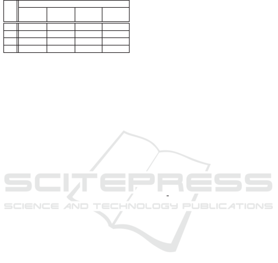
Table 5: Rank correlation coefﬁcient.

Sur

(p) Sur

(p)

0.9974 0.9999 0.9990 0.9999

0.9155 0.9972 0.9516 0.9611

0.9958 0.9999 0.9999 0.9999

0.9913 0.9998 0.9902 0.9976

’ P

’: P

It is clearly demonstrated that linear

approximations,Sur

(p) and Sur

(p), are much

less accurate than more complicated approximations,

Sur

(p) and Sur

(p). It illustrated that there are

interesting interactions among age groups. We also

conﬁrmed that if the training set and testing set are

very different, the performance of Sur

(p) is less

impressive than Sur

(p). However, when the training

set does contain similar points as testing set, Sur

(p)

outperforms Sur

(p). It is more accurate and has

higher rank coefﬁcient correlation.

Our results conﬁrm the ﬁnding of previous studies

that school children should be vaccinated with high

priority. One obvious future direction is to use ma-

chine learning to explore the vast landscape of scenar-

ios with various objective functions and constraints.

For example, the infectiousness of the virus strand

might vary, the available date of vaccine may not

be known in advance, and other mitigation strategies

such as antiviral treatment and school closure might

vary. The objective function can vary too. Instead of

minimizing infected cases, one might want to mini-

mize economic cost (Meltzer et al., 1999). Currently,

we the only variables are the amounts of vaccine al-

located to different age groups. More parameters will

be included as input and we plan to try the convo-

lutional neural network and the recurrent neural net-

work in the future. We hope not only we can con-

struct accurate surrogates with more parameters, but

also can gain insight about the delicate interaction be-

tween model parameters and outcome by studying the

neural networks.

Finally, we envision that an autonomous software

searches through the huge scenario space with the

help of surrogate function and adaptively executes

simulation program to revise the surrogate function

to produce higher ﬁdelity surrogate and better search

results by applying reinforcement learning methods.

ACKNOWLEDGEMENTS

We thank anonymous reviewers for their sugges-

tions. The research is partially funded by the grant of

”MOST105-2221-E-001-034”, ”MOST104-2221-E-

001-021-MY3”, and ”Multidisciplinary Health Cloud

Research Program: Technology Development and

Application of Big Health Data. Academia Sinica,

Taipei, Taiwan”.

REFERENCES

Basta, N. E., Halloran, M. E., Matrajt, L., and Longini, I. M.

(2008). Estimating inﬂuenza vaccine efﬁcacy from

challenge and community-based study data. Ameri-

can Jourmal of Epidemiology, 168(12):1343–1352.

Chang, H.-J., Chuang, J.-H., Fu, Y.-C., Hsu, T.-S., Hsueh,

C.-W., Tsai, S.-C., and Wang, D.-W. (2015). The im-

pact of household structures on pandemic inﬂuenza

vaccination priority. In Proceedings of the 5th In-

ternational Conference on Simulation and Modeling

Methodologies, Technologies and Applications - Vol-

ume 1: SIMULTECH,, pages 482–487.

Chao, D. L., Halloran, M. E., Obenchain, V. J., and Longini,

Jr, I. M. (2010). Flute, a publicly available stochastic

inﬂuenza epidemic simulation model. PLOS Compu-

tational Biology, 6(1):1–8.

Clevert, D., Unterthiner, T., and Hochreiter, S. (2015). Fast

and accurate deep network learning by exponential

linear units (elus). CoRR, abs/1511.07289.

Dozat, T. (2015). Incorporating nesterov momen-

tum into adam. http://cs229.stanford.edu/proj2015/

054

report.pdf.

Fu, Y.-c., Wang, D.-W., and Chuang, J.-H. (2012). Rep-

resentative contact diaries for modeling the spread of

infectious diseases in taiwan. PLoS ONE, 7(10):1–7.

Germann, T. C., Kadau, K., Longini, I. M., and Macken,

C. A. (2006). Mitigation strategies for pandemic in-

ﬂuenza in the United States. Proceedings of the Na-

tional Academy of Sciences, 103(15):5935–5940.

Gosavi, A. (2015). Simulation-based optimization. para-

metric optimization techniques and reinforcement

learning.

Jian, Z.-D., Hsu, T.-S., and Wang, D.-W. (2016). Search-

ing vaccination strategy with surrogate-assisted evo-

lutionary computing. In Proceedings of the 6th In-

ternational Conference on Simulation and Modeling

Methodologies, Technologies and Applications - Vol-

ume 1: SIMULTECH,, pages 56–63.

Jin, Y. (2011). Surrogate-assisted evolutionary computa-

tion: Recent advances and future challenges. Swarm

and Evolutionary Computation, 2(1):61–70.

J.J. Grefenstette, J. F. (1985). Genetic search with approxi-

mate ﬁtness evaluations. In International Conference

on Genetic Algorithms and Their Applications, pages

112–120.

Keras (2015). Keras documentation. https://keras.io/.

Loshchilov, I., Schoenauer, M., and Sebag, M. (2010).

Parallel Problem Solving from Nature, PPSN XI:

11th International Conference, Krak´ow, Poland,

Learning from Simulated World - Surrogates Construction with Deep Neural Network

September 11-15, 2010, Proceedings, Part I, chap-

ter Comparison-Based Optimizers Need Comparison-

Based Surrogates, pages 364–373. Springer Berlin

Heidelberg, Berlin, Heidelberg.

Meltzer, M. I., Cox, N. J., and Fukuda, K. (1999). The

economic impact of pandemic inﬂuenza in the United

States: priorities for intervention. Emerging Infect.

Dis., 5(5):659–671.

Tsai, M.-T., Chern, T.-C., Chuang, J.-H., Hsueh, C.-W.,

Kuo, H.-S., Liau, C.-J., Riley, S., Shen, B.-J., Shen,

C.-H., Wang, D.-W., and Hsu, T.-S. (2010). Efﬁcient

simulation of the spatial transmission dynamics of in-

ﬂuenza. PLOS ONE, 5(11):1–8.

SIMULTECH 2017 - 7th International Conference on Simulation and Modeling Methodologies, Technologies and Applications