Mobility Strategies based on Virtual Forces for Swarms of
Autonomous UAVs in Constrained Environments
Ema Falomir
1,2
, Serge Chaumette
1
and Gilles Guerrini
2
1
Bordeaux Computer Science Research Laboratory, Bordeaux University, Talence, France
2
Thales Systèmes Aéroportés, Mérignac, France
Keywords: UAV, Swarm, Autonomous Swarm of UAVs, Compactness, Virtual Forces, Distributed Robotic Systems.
Abstract: The usage of autonomous unmanned aerial vehicles (UAVs) has recently become a major question. For
wide area surveillance missions, a swarm of UAVs can be much more efficient than a single vehicle. In this
case, several aircrafts cooperate in order to fulfill a mission while avoiding collisions between each other
and with obstacles. This article proposes original distributed mobility strategies for autonomous swarms of
UAVs, the goal of which is to fulfill a surveillance mission. Our work is based on virtual forces and our
approach allows narrow areas crossing that require a compact formation of the autonomous swarm.
1 INTRODUCTION
In the past few years, the usage of unmanned aerial
vehicles (UAVs) has been widely studied. In this
paper, we consider rotor wings, which allow low
speed maneuvering and hovering.
A set of several UAVs deployed on the same
area, independent of any infrastructure and able to
establish peer-to-peer connections form a flying ad-
hoc network (FANET) (Bekmezci et al., 2013). A
FANET offers several advantages in comparison to a
single UAV. Additionally to a larger coverage, if
one aircraft of a FANET encounters a failure, the
assigned mission can still be achieved. Furthermore,
each UAV can embed a different sensor, which
could not fit inside a single aircraft.
Several studies have already been carried out on
surveillance missions lead by FANETs. The UAVs
can all be multirotors (Chaumette et al., 2011) but
multirotors also can be associated with fixed-wings
(Jaimes et al., 2008), (Bouvry et al., 2016).
In this paper, we will consider a FANET
composed of multirotors with the same kinematics
characteristics, able to fulfill a mission
autonomously. We will refer to this particular kind
of FANET as “autonomous swarm”. In this
configuration, an operator only deals with a single
entity contrary to a multiplatform system.
To evolve in partially unknown environment
autonomously, the UAVs have to calculate their
flight plans online. Here, not to be dependent of a
single UAV, each one calculates its own flight plan.
Methods based on artificial potential fields
(introduced in (Khatib, 1986)) are often chosen for
online and decentralized applications thanks to their
limited needs in terms of computation and because
they are distributed by nature. They can be used to
maximize area coverage (Howard et al., 2002),
(Gobel and Krzesinski, 2008) or to obtain specific
connectivity characteristics (Casteigts et al., 2012).
Some studies also aim at reaching a target with robot
cars thanks to artificial forces approaches
(Boonyarak and Prempraneerach, 2014), (Jin et al.,
2014) but these methods have not been widely
extended to swarms.
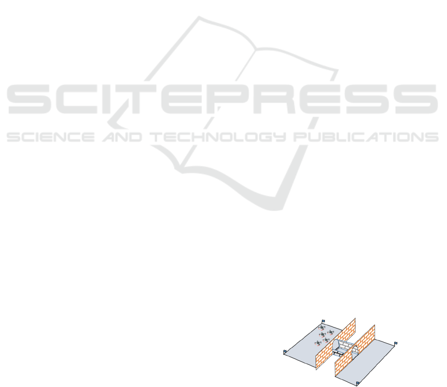
In this paper, we consider a cooperative and
autonomous swarm of multirotors in the context of a
surveillance mission of two areas of interest (AoIs),
as represented on the Figure 1. The two AoIs are
separated by a narrow passage (a tunnel), possibly
containing static obstacles of unknown position and
size, requiring a compact formation of the swarm.
Figure 1: Representation of the two Areas of Interest
separated by a narrow passage (a tunnel).
Falomir E., Chaumette S. and Guerrini G.
Mobility Strategies based on Virtual Forces for Swarms of Autonomous UAVs in Constrained Environments.
DOI: 10.5220/0006418202210229
In Proceedings of the 14th International Conference on Informatics in Control, Automation and Robotics (ICINCO 2017), pages 221-229
ISBN: 978-989-758-263-9
Copyright
c
2017 by SCITEPRESS – Science and Technology Publications, Lda. All rights reserved
We propose a new distributed mobility strategy
for autonomous swarms of UAVs, based on virtual
forces in order to avoid collisions between the
UAVs and with obstacles, and maximize the
communication links along a surveillance mission.
The remainder of this paper is organized as
follows. Section 2 presents the scenario and the
associated hypothesis. Section 3 introduces the
forces used in the mobility strategies thereafter
presented in section 4. Section 5 introduces the
metrics used to evaluate the efficiency of our
mobility strategies. The results are shown in section
6. Finally, section 7 is dedicated to the conclusion of
this work and sketches future research directions.
2 SCENARIO AND HYPOTHESIS
Scenario
Our mission aims at the successive surveillance, by
an autonomous swarm of UAVs, of two AoIs
separated by a narrow passage possibly containing
obstacles unknown prior to the mission. The UAVs
are multirotors equipped with limited range sensors
supporting the surveillance mission and allowing
obstacle detection and with communication systems.
Hypothesis
We suppose that there are no obstacles in the AoIs
but only in the narrow passage which is the phase of
the scenario that we want to study in details. We also
assume consider that the UAVs know the
coordinates of the AoIs corners and of the passage
entrance. Additionally, it is supposed that no UAV is
added or removed from the system.
As we are interested in mobility strategies, we do
not consider neither “low-level” details in this first
study (communication protocols, localization, etc.)
nor the UAVs flight dynamics. Moreover, it is
supposed that the UAVs have enough energy to
fulfill the complete mission.
3 CONTRIBUTION 1: VIRTUAL
FORCES
To achieve a surveillance mission and to avoid
collisions, mobility strategies are proposed based on
virtual forces and on distances of interest which are
presented in the following subsections.
For this study, we have chosen to define the
forces with a magnitude comprised between -1 and
1. Attractive forces are positive, repulsive forces are
negative. This permits to easily compare the
influence of several forces in a system which can be
complex. Moreover, as this is a preliminary study,
forces are defined on the basis of linear functions.
Safety Distance
In order to avoid collisions, a minimal safety
distance, D
has to be maintained between each
UAV and other objects. For this preliminary study,
we define this distance as follows:
1.5
(1)
Inter-UAV Wanted Distance
During the mission, two goals must be achieved.
First, the maintenance of the communication links,
and second the coverage of the AoI with little
redundancy. Consequently, we define an inter-UAV
wanted distance which takes into account the
communication and the surveillance sensor ranges:
min
2
,
(2)
where k∈
0;1
.
It is important to note that D
must be greater
than (or equal to) D
to use the strategy described
in the following sections. In practice, this condition
is not limiting as UAVs always embed sensors with
range larger than their own size.
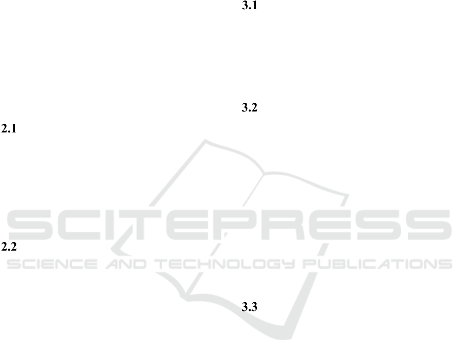
Attraction-repulsion between UAVs
To fulfill their mission, the UAVs should remain
spaced of D
. In this aim, an attractive force is
applied when they are further and a repulsive one
when they are closer, depending on their distance
d
. As the UAVs safety is more important than the
mission accomplishment, the repulsive forces have
to be stronger than the attractive ones. The
attractive-repulsive virtual forces between UAVs are
directed from the considered UAV to its neighbor
and of magnitude F
(see Figure 2) defined in (3).
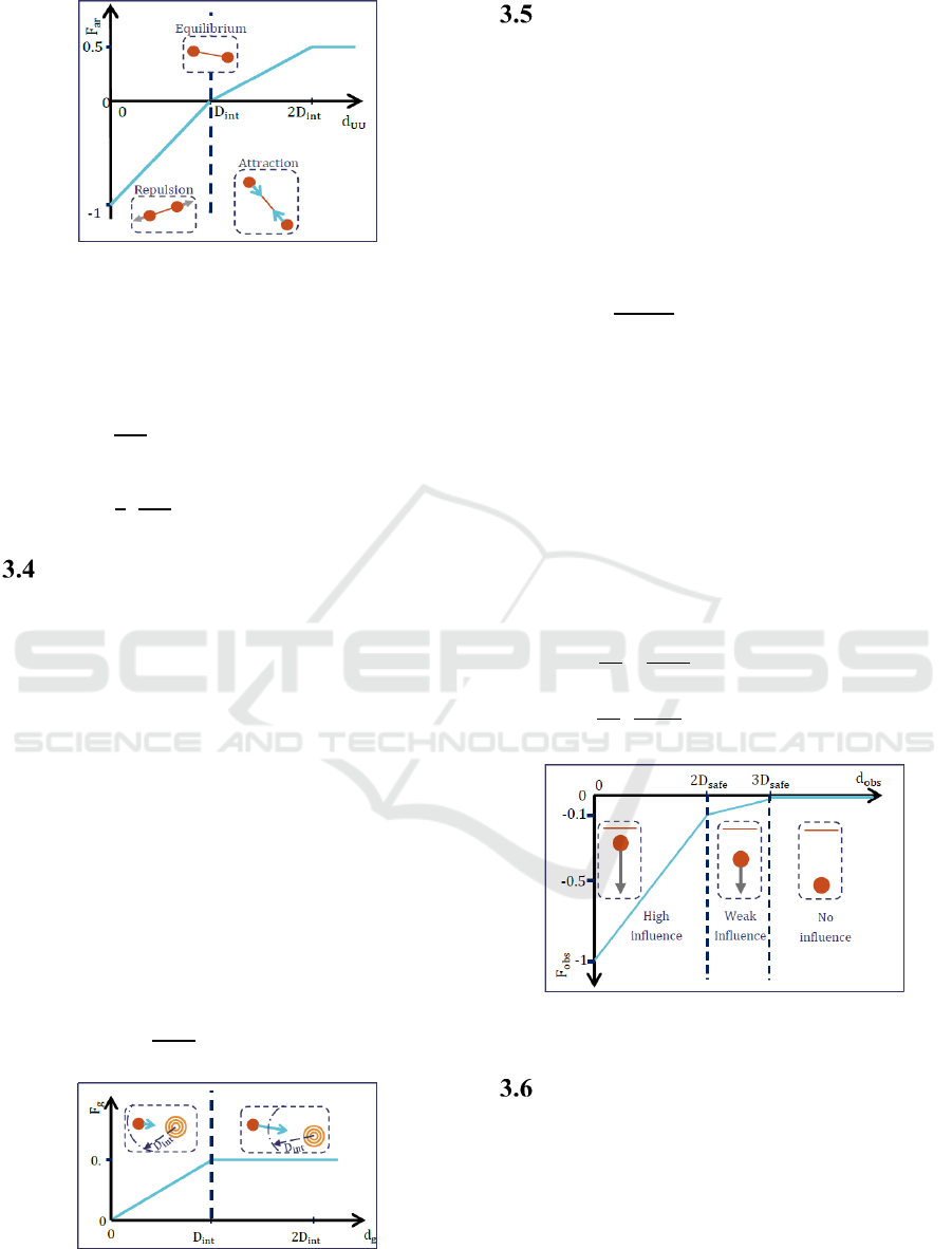
Figure 2: Graphical representation of the attractive-
repulsive force between UAVs. On the schemes, UAVs
are represented by discs, attractive and repulsive forces are
represented by open and triangle arrows respectively. The
lines linking the UAVs represent communication links.
Note: These notations will be used all along the paper.
1
1 i
f
0.5 if
2
1
2
1
(3)
Attraction towards a Goal
To fulfill the mission, the UAVs have to deploy on
the AoIs, fly over them, and cross the passage. To
achieve these goals, each UAV calculates temporary
targets all along the mission and is subject to an
attractive force towards them.
We have chosen to give a constant magnitude to
the attractive force towards a goal till a certain
distance. In the area around the target, the force
decreases linearly with respect to the robot-goal
distance d
, in order to avoid oscillations around the
goal. This decrease near the target also favors the
other forces in this area.
The attraction to a goalis directed towards the
goal and is of magnitude F
(represented on Figure
3) defined as follows:
0.5 i
f
2
else
(4)
Figure 3: Graphical representation of the attractive force to
a goal. The UAV target is represented by nested circles.
Note: This notation will be used all along this paper.
Repulsion Due to Obstacles
The repulsion due to obstacles is based on the safety
distance D
. In this first study, we admitted that if
a UAV is further away than three times its safety
distance from an obstacle, it should not consider the
obstacle. Nonetheless, in future work this repulsive
force should be based on other characteristics.
The repulsive force due to an obstacle is directed
at the opposite of the obstacle. A first magnitude has
been tested, F
, defined as follows:
3
1 if
3
0else
(5)
where d
is the UAV-obstacle distance. Using this
first approach, the repulsion due to obstacles was too
high compared to the attraction-repulsion between
UAVs. As a result, the swarm did not remain
connected in the tunnel, and collisions between
UAVs occurred. Indeed, between 2D
and 3D
,
the obstacle had a too high influence. So we
modified the magnitude to F
, represented in the
Figure 4, defined as follows:
0if
3
9
20
1 if
2
1
10
3 else
(6)
Figure 4: Graphical representation of the repulsive force
due to obstacles. The obstacle is represented by a line.
Weighted Average
At each step, each UAV is subject to several virtual
forces as illustrated on the Figure 5. UAVs calculate
a weighted average of all the virtual forces applied
to them and their next direction is resulting of this
weighted average. The weight of each force is the
exponential of its magnitude, as proposed for spring
forces in a work on network biconnection (Casteigts
et al., 2012).
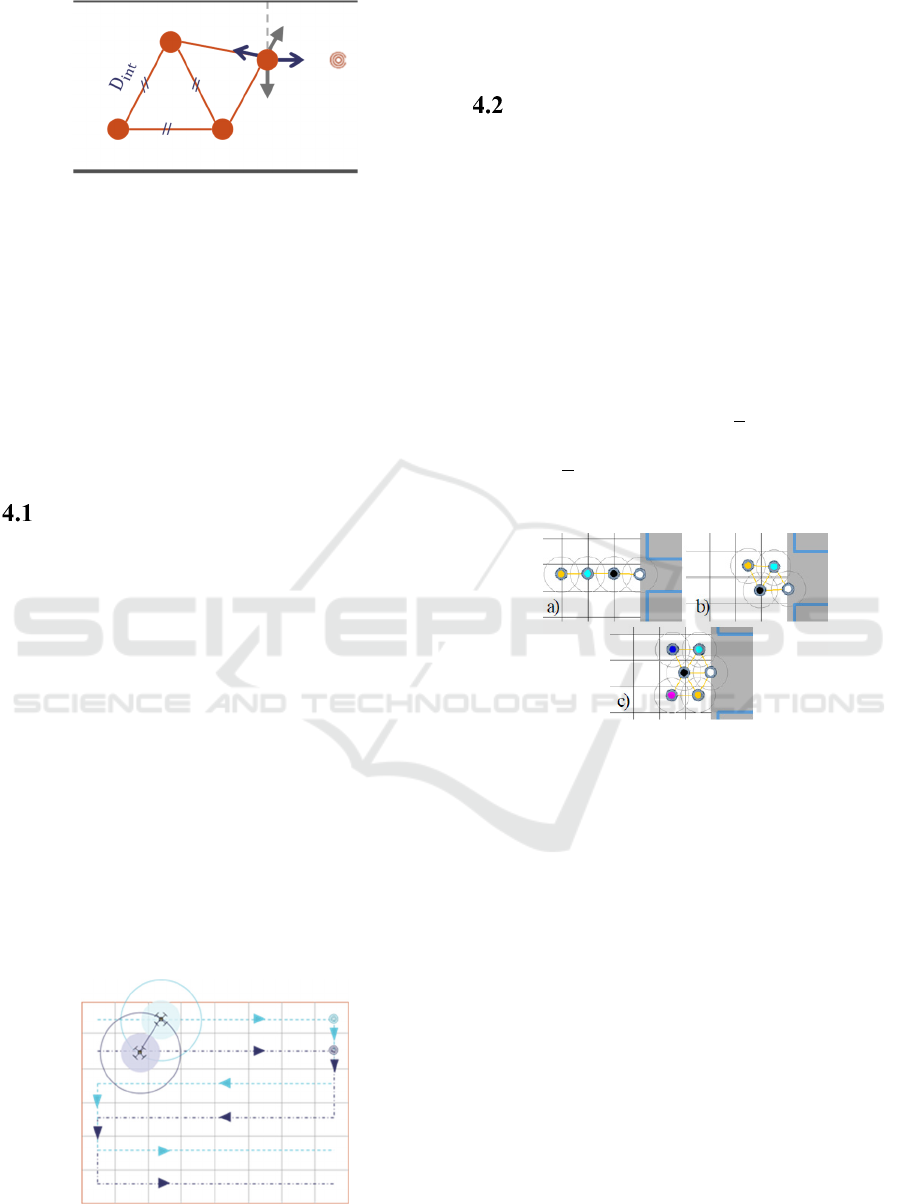
Figure 5: Scheme of the repulsive and attractive forces
applied to a UAV in a swarm, in a narrow passage.
4 CONTRIBUTION 2: MOBILITY
STRATEGIES
As introduced in section 2, our scenario is composed
of three main phases: survey the AoIs, make-up of
the compact formation and cross the tunnel. In the
following subsections we detail the mobility
strategies for each of these three steps.
Surveillance Mobility Strategy
During the surveillance phase, each UAV should
have, at each moment, a vision of the whole AoI as
recent as possible. To be able to build this view in a
cooperative manner, the UAVs have to be deployed
all over the area and maintain communication links.
An adapted mobility strategy consists in creating
an “S-shaped” travel over the AoI, as illustrated in
Figure 6. The mesh to support the movements of the
UAVs is calculated at the very beginning of the
mission and is composed of cells of size D
D
.
In this mobility strategy, the targets of the UAVs
are located at the extremity of the lines. Once a
UAV reaches its temporary goal, it calculates its
next target, depending on its identifier and of the
number of vehicles in the swarm. Its move towards
this target starts when its 1- and 2-hop neighbors
have reached their own goals. In this way, the
connectivity of the swarm is maintained.
Figure 6: Movements of a swarm composed of two UAVs
during the surveillance mission over an AoI.
During the surveillance, each UAV is subject to
attractive-repulsive force with its neighbors and to
attractive force towards its successive targets.
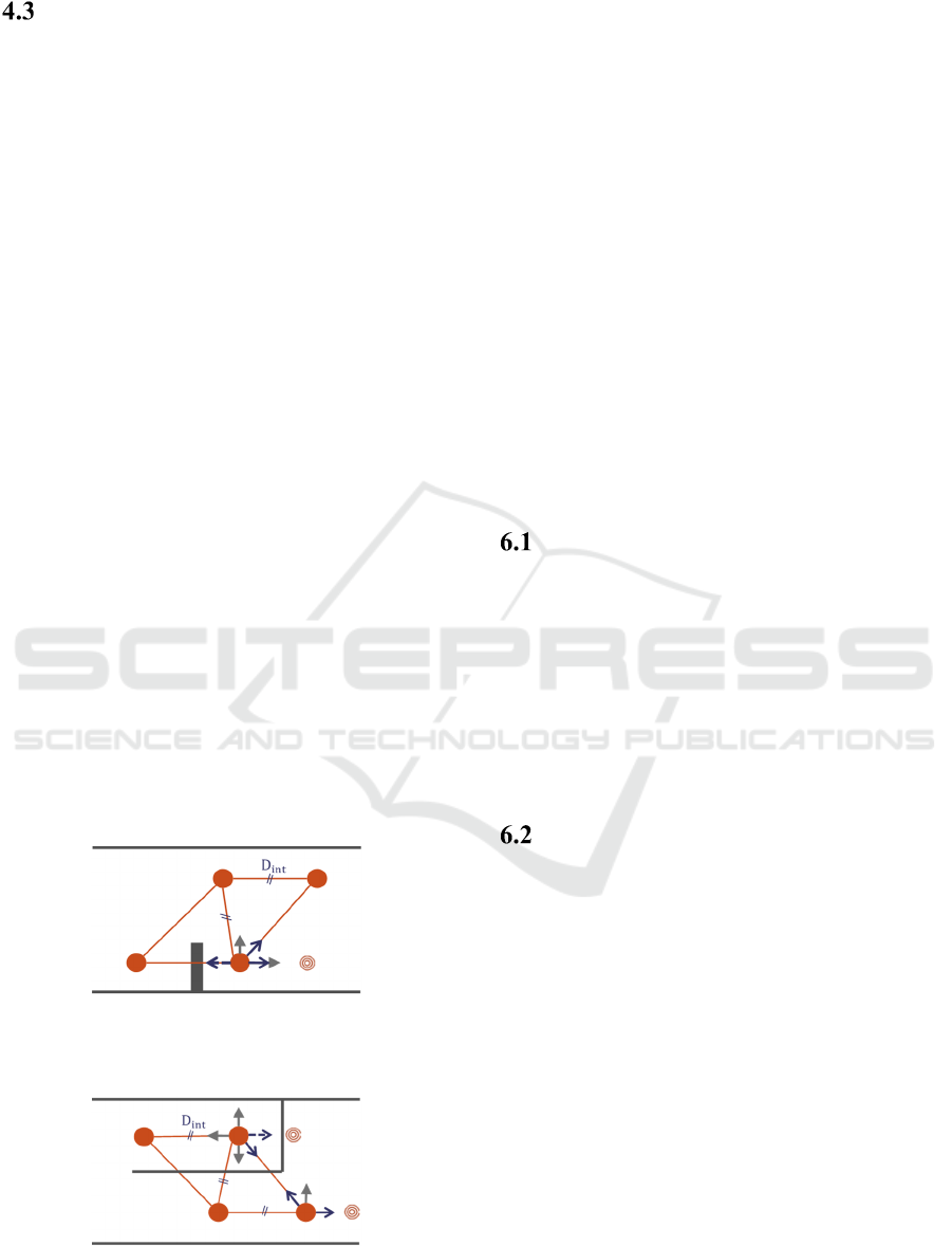
Compact Swarm Formation Setup
Once the first AoI has been covered, the swarm flies
toward the passage in which it can encounter
obstacles. In this study, the UAVs do not share the
obstacles location, but in a further work this should
be implemented. To facilitate this, a biconnectivity
of the swarm is sought. In case of a very narrow
passage (i.e. of a width smaller than 3D
), UAVs
can only get through the tunnel in a queue (Figure 7
a), so biconnectivitv cannot be guaranteed. Else, the
swarm can organize itself in a staggered rows
formation (see Figure 7 b) and c)). The 2-row
staggered formation can be setup when the passage
width is greater than 2D
√
3/2D
. To allow 3
rows, the tunnel width has to be greater than
2D
√
3D
. These values can easily be
geometrically calculated.
Figure 7: a) Too narrow passage for a biconnectivity. This
will be referred to as Tunnel shape a. b) 2-row staggered
biconnected formation. (Tunnel shape b.) c) Biconnected
formation for larger passages. (Tunnel shape c.).
From the passage width, the number of vehicles
in the swarm and its identifier, each UAV calculates
a target close to the tunnel entrance, in a
deterministic manner. The connectivity of the swarm
during the surveillance ensures that all the UAVs
know when they have to go towards the tunnel
entrance. The positions of the UAVs in compact
formation are separated of D
, so there will be
some communication links between the UAVs. So,
only the repulsive forces between the UAVs and
thee attractive force to their goal are necessary when
the swarm travels towards the tunnel entrance. The
swarm starts to get through the passage only when
all the UAVs are at their position or when UAVs are
at their correct location for a defined duration.
Passage Crossing Mobility Strategy
The swarm has to cross the tunnel to reach the
second AoI.
When the UAVs get through the tunnel, they are
subject to the virtual attractive-repulsive forces
between each other, the repulsive force due to the
obstacles and the attractive force towards a goal. As
the UAVs do not know the shape of the passage,
they calculate at each step a new temporary target in
the direction of the second AoI. This target is
located at a small distance (we arbitrarily chose
D
/4) and so produces a weak attraction, the goal
being to favor collision avoidance and to maintain of
the communication links.
If an obstacle is located between the UAV and its
target, the UAV stops being attracted towards this
point and it favors the attraction towards its
neighbors so as not to stay in a local minima.
We consider that the UAVs can communicate
even if an obstacle is located between them.
Additionally, if a UAV shares a communication link
with another one in the opposite direction of its
target and if an obstacle is between them, the first
UAV will not take into account the attractive force
towards this neighbor (see Figure 8). A further
simplification is made in this first study concerning
the repulsion due to obstacles. Each UAV
decomposes its environment in four equal areas:
upper, below, backwards and ahead. They take into
account a maximum of one repulsive force due to
obstacles in each quadrant. If several obstacles are in
a same quadrant, the closest one only is taken into
account. This is enough to avoid obstacles.
Figure 8: Case when an attractive force is not taken into
account (dotted open arrow). The forces are plotted for the
UAV of interest.
Figure 9: A limitation of the model. The forces are plotted
for only two UAVs for the sake of visibility. The two
upper UAVs do not go backward for joining the others.
Nonetheless, limitations exist. Indeed, there is no
definition of a new target if there is an obstacle
between it and the UAV, and favoring the attraction
towards other UAVs is not always sufficient as
illustrated on Figure 9.
5 EVALUATION CRITERIA
The presents the Measures of Performance (MoPs)
for the three parts of the scenario. For each MoP, an
ideal result is given, not always achievable.
6 SIMULATION AND RESULTS
The following subsections present the simulation
tool used in this study, the parameters of the
simulations and the results for the different steps,
according to the MOPs defined in section 5.
JBotSim Simulation Tool
To simulate the mobility strategies defined in the
previous section, we chose the open source
simulation library JBotSim (Casteigts, 2015). It is a
tool for distributed algorithms fast prototyping in
dynamic networks. Contrary to other well-known
simulators such as NS3 (Riley and Henderson, 2010)
or OMNet++ (Varga, 2001), JBotSim does not
implement real-world networking protocols, which
was not required in this preliminary study.
Simulation Scenario and
Parameters
We have conducted a series of simulation to validate
our mobility strategies. For all the simulations the k
factor used in the D
definition is fixed at 0.75.
We chose to simulate UAVs of circular shapes of
20cm diameter, equipped with a communication
system of 1.10m range and with a sensor used for
both surveillance and obstacle detection of 50cm
range.
The first AoI is 9m long and 7.50m large. At
each simulation step, the UAVs travel at a random
distance comprised between 5cm and 10cm in the
resulting direction of the virtual forces average.
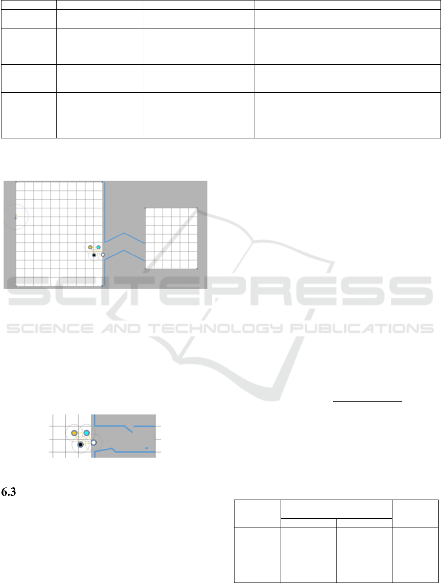
Table 1: Evaluation criteria and ideal result for each step of the mission.
Operational Objective MoPs Ideal Result
Overall
mission
Safeguard of the UAV
Distance between a UAV
and another objec
t
Greater than a given safety distance
Surveillance
mission
Deploy over the AoI
with communication
links
Duration of an AoI coverage
Number of disconnections
Number of connections
Inversely proportional to the number of UAVs
None
Equal to the number of disconnections
Compact
formation
setup
Quick set up before
crossing the tunnel
Duration of compact
formation setup
Time of travel between the furthest UAV and the
tunnel entrance, by the shortest path
Tunnel
crossing
Join the second AoI
while avoiding
collisions
Duration of tunnel crossing
Number of network
disconnections
Number of network re-
connections
Time of travel of one UAV in the tunnel by the
shortest path
None
Equal to the number of disconnections
A view of the AoIs, tunnel and UAVs extracted
from JBotSim is shown on the Figure 10.
Figure 10: View of the two AoIs and of the passage
referred to as Tunnel d.
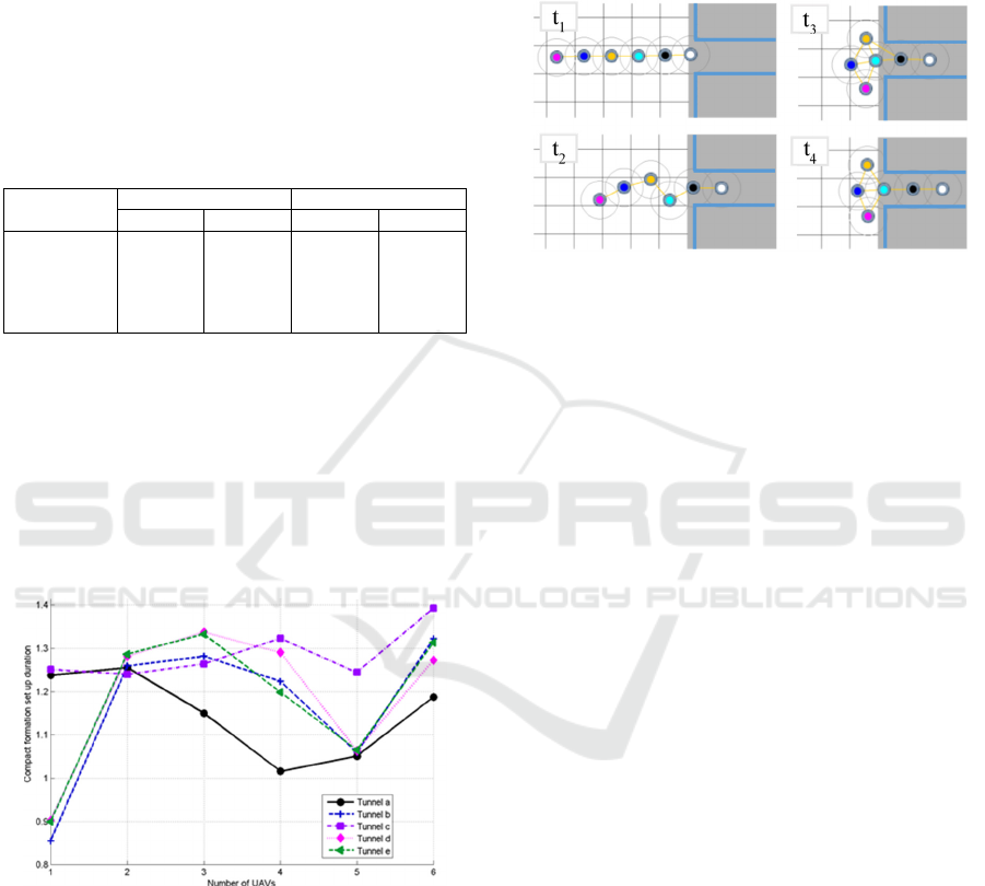
Simulations have been performed with swarms
composed of 1 to 6 UAVs and with 5 tunnels (see
Figure
7, Figure 10 and Figure 11). For each
parameter set we have run 30 simulations. At the
entrance, shape a tunnel is 95cm large, tunnels b, d
and e are 151cm large and finally tunnel c is 226cm
large.
Figure 11: Passage referred as Tunnel e.
Simulation Results, Evaluation and
Analysis
6.3.1 Overall Mission
During the whole mission, the priority is to
safeguard the UAVs. To achieve this goal, the
distance between a UAV and another object has to
remain above the safety distance defined previously.
The minimal distance between the UAVs as well
as between the UAVs and an obstacle, remained
above 1.3 timesD
, for all the simulation ran.
Thus, the main objective of the project is reached.
6.3.2 Surveillance
As expected, the simulations have shown that the
more UAVs compose the swarm, the quicker the
complete surveillance is performed (see Table 2).
The very small difference of duration between 4
and 5 UAVs is due to the number of rows of the
mesh supporting the UAVs movements in the AoI.
Indeed, a 4-UAV swarm has to cross the 12-row
area three times to fully cover it, as a 5-UAV
swarm.
Furthermore, a UAV moves towards its next
target only when its neighbors have reached their
own one. Indeed the more UAVs compose the
swarm, the higher is the probability to have to wait
for other UAVs. This is why the speed-up, defined
as follows, is not linear:
SpeedUpnUAVs
duration1UAV
duration
nUAVs
(7)
Even if the objective of measuring a linear speed-up
is not reached, we can observe a clear decrease in
duration when the number of UAVs increases.
Table 2: Mean and standard deviation (SD) of the first AoI
surveillance duration for various numbers of UAVs in the
swarm, calculated on 150 runs for each number of UAVs.
Number of
UAVs
Duration of surveillance
(number of steps)
Speed Up
Mean SD
1 1210 7 1
2 764 14 1.6
3 555 5 2.2
4 425 8 2.8
5 416 4 2.9
6 233 11 5.2
Finally, as the mobility strategy for the
surveillance phase is almost deterministic (random
speed of the UAVs), the standard deviation is low
and so an estimation of the surveillance duration can
be done by running a configuration only once.
Furthermore, we studied the creation and loss of
links during the surveillance step (see the values in
Table 3). We can see that there are on average a few
loss of links, and as many creation as loss. The
objective for this MOP is thus reached.
Table 3: Mean and standard deviation (SD) of the number
of links lost and created during the surveillance phase,
calculated on 150 runs for each number of UAVs.
Number of
UAVs
Lost Links Created Links
Mean SD Mean SD
2 0.05 0.26 0.05 0.26
3 0.09 0.29 0.09 0.30
4 0.77 2.33 0.76 2.32
5 2.03 4.80 2.02 4.77
6 3.51 5.41 4.49 5.32
6.3.3 Compact Formation Setup
The Figure 12 shows the duration between the end
of the surveillance and the moment when the
compact formation is set up, normalized by the
necessary time to go from the further UAV position
to the tunnel entrance. As UAV target is not exactly
at the tunnel entrance, the normalization can be
smaller than one.
Figure 12: Mean compact formation setup duration for
each simulated configuration, normalized.
Width of tunnel shape b, d and e are the same, so
we wait for an identical duration of compact
formation setting up. Nevertheless, differences
appear between the 3 curves, due to the zoom effect.
In the case of a single UAV, the duration is the
smallest for all the tunnels, because there is no
repulsive force with neighbors, and so the UAV is
not subject to forces opposed to the target attraction.
For all the configurations, the normalized
compact formation setup duration is smaller than
1.4, which is a good result. This means that even for
a swarm composed of numerous UAVs, and
independently of the compact formation shape, the
formation setup is rather quick.
Figure 13: Movements of a 6-UAV swarm aiming at
entering in the tunnel. At the time t
, the swarm is in a
local equilibrium at the tunnel entrance.
We note that we tried to simulate a thinner width
for Tunnel shape a (of width 2D
instead of
3D
). In this case, only multi-UAVs swarms
entered: for a single UAV, the repulsive forces at the
entrance of the tunnel were greater than the
attractive force towards the target. In the case of
several UAVs, the attraction-repulsion between
them was in the same direction as the attraction
towards their target, which allowed the swarm to
enter in the tunnel. Nevertheless it occurred that a 6-
UAV swarm reached a local equilibrium at the
passage entrance (see the progression of the swarm
on Figure 13). In the case of such equilibrium, the
closest UAVs to the tunnel were slowed down
because of the repulsion due to the walls, while the
other UAVs had a strong attraction towards their
target and so did not remain behind the others.
6.3.4 Tunnel Crossing
The duration of tunnel crossing is the duration
between the entrance of the first UAV and the exit
of the last one. Results are represented in Figure 14.
The tunnel crossing duration for the thinner
tunnel does not vary in function of the number of
UAVs. This is because the UAVs have to be queued
in this case and so the attractive-repulsive forces
between them are in the direction of their target.
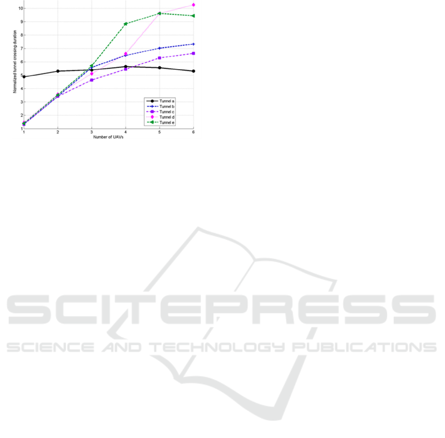
Figure 14: Tunnel crossing duration for each simulated
configuration, normalized by the duration of tunnel
crossing by a single UAV by the shortest path at
maximum speed.
As expected, tunnels of shape b and c show the
same trend even if the largest one is crossed quicker.
We note that in the case of several UAVs and
tunnel of shape b to e, the crossing duration is longer
than for a single UAV. This is due to the attractive-
repulsive forces between the UAVs which are not in
the direction of their target.
For the tunnel shape d, the crossing duration
follows the trend of tunnel shapes b and c until 4
UAVs and skyrockets for 5 UAVs. This is due to the
creation of additional links between the UAVs
during the travel through the linear parts which have
to be broken to pass over the corner.
In the case of the tunnel shape e, we can notice a
strong increase of the crossing duration from 4
UAVs, due to the two obstacles which are too close
to allow a biconnectivity. For that reason, some links
between the UAVs have to be broken, while an
attractive force between them is still applied. From 4
UAVs, two links have to be broken and only one in
the case of 3 UAVs.
Moreover, in all the simulations, the connectivity
of the swarm was maintained in the tunnel.
7 CONCLUSIONS AND FUTURE
WORK
In this paper we propose original mobility strategies
based on virtual forces for a swarm of autonomous
UAVs. Following these strategies, the UAVs, all
having equivalent roles, can autonomously fulfill a
surveillance mission of two AoIs separated by a
narrow passage. To travel from the initial AoI to the
other, the swarm organizes itself as a compact
formation favoring communication links between
the UAVs, which travel through the tunnel while
avoiding obstacles unknown prior to the mission.
We have run many simulations and evaluated
them using a number of criteria. Our results show
that our approach gives very good results.
Nevertheless, numerous topics have to be further
explored. First of all, the UAV safety distance
should depend on the range of the embedded sensor
used to detect the obstacles, as well as on the speed
of the UAVs. Furthermore, each UAV that detects
an obstacle should share its location with the other
aircrafts of the swarm. Thanks to this information,
the UAVs could calculate a new target points taking
the obstacle into consideration. The presence of
obstacles on the AoI could also be considered. A
wide subject of study could be the self-organization
of the swarm in order to make up a compact
formation depending on the tunnel width, instead of
the deterministic configuration presented in this
work. Finally, magnitudes of the three forces could
be defined by other functions, as polynomial or
exponential. This could improve the model strategies
by speeding up surveillance or tunnel crossing.
REFERENCES
Al Redwan Newaz, A., Lee, G., Adi Pratama, F. & Young
Chong, N., 2013. 3D Exploration Priority Based
Flocking of UAVs. Takamatsu, Japan, IEEE, pp. 1534-
1589.
Autefage, V., Chaumette, S. & Magoni, D., 2015. A
Mission-Oriented Service Discovery Mechanism for
Highly Dynamic Autonomous Swarms of Unmanned
Systems. s.l., IEEE, pp. 31-40.
Bekmezci, I., Sahingoz, O. K. & Temel, S., 2013. Flying
Ad-Hoc Networks (FANETs): A survey. Ad Hoc
Networks, May, 11(3), pp. 1254-1270.
Boonyarak, S. & Prempraneerach, P., 2014. Real-Time
Obstacle Avoidance for Car Robot Using Potential
Field and Local Incremental Planning. Nakhon
Ratchasima, Thailand, IEEE.
Bouvry, P. et al., 2016. Using heterogeneous multilevel
swarms of UAVs and high-level data fusion to support
situation management in surveillance scenarios.
Baden-Baden, IEEE, pp. 424-429.
Cakir, M., 2015. 2D Path Planning of UAVs with Genetic
Algorithm in a Constrained Environment. Istanbul,
Turkey, IEEE.
Camp, T., Boleng, J. & Davies, V., 2002. A survey of
mobility models for ad hoc network research. Wireless
Communications and Mobile Computing, August,
2(5), pp. 483-502.
Casteigts, A., 2015. JBotSim: a Tool for Fast Prototyping
of Distributed Algorithms in Dynamic Networks.
Athens, Greece, s n.

Casteigts, A. et al., 2012. Biconnecting a Network of
Mobile Robots using Virtual Angular Forces.
Computer Communications, 35(9), pp. 1038-1046.
Chaumette, S. et al., 2011. CARUS, an operational
retasking application for a swarm of autonomous
UAVs: First return on experience. s.l., IEEE.
Gobel, J. & Krzesinski, A. E., 2008. A Model of
Autonomous Motion in Ad Hoc Networks to Maximise
Area Coverage. Adelaide, Australia, IEEE.
Howard, A., Mataric, M. J. & Sukhatme, G. S., 2002.
Mobile Sensor Network Deployment using Potential
Fields: A Distributed, Scalable Solution to the Area
Coverage Problem. Fukuoka, Japan, Springer.
Jaimes, A., Kota, S. & Gomez, J., 2008. An approach to
surveillance an area using swarm of fixed wing and
quad-rotor unmanned aerial vehicles UAV(s). s.l.,
IEEE.
Jin, J., Adrian, G. & Gans, N., 2014. A Stable Switched-
System Approach to Obstacle Avoidance for Mobile
Robots in SE(2). Chicago, IL, USA, IEEE, pp. 1533-
1539.
Khatib, O., 1986. Real-Time Obstacle Avoidance for
Manipulators and Mobile Robots. The International
Journal of Robotics, 03 01, 5(1), pp. 90-98.
Riley, G. F. & Henderson, T. R., 2010. The ns-3 Network
Simulator. Dans: K. Wehrle, M. Güneş & J. Gross,
éds. Modeling and Tools for Network Simulation.
s.l.:Springer Berlin Heidelberg, pp. 15-34.
To, L., Bati, A. & Hillard, D., 2009. Radar Cross Section
measurements of small Unmanned Air Vehicle Systems
in non-cooperative field environments. s.l., IEEE, pp.
3637-3641.
Varga, A., 2001. The OMNeT++ discrete event simulation
system. Prague, Czech Republic, s n., pp. 319-324.
