
Dynamic Stability of Repeated Agent-Environment Interactions During
the Hybrid Ball-bouncing Task
Guillaume Avrin
1,2,3
, Maria Makarov
1
, Pedro Rodriguez-Ayerbe
1
and Isabelle A. Siegler
2,3
1
Laboratoire des Signaux et Syst
`
emes (L2S), CentraleSup
´
elec - CNRS - Univ. Paris-Sud, Universit
´
e Paris-Saclay,
Plateau du Moulon, 3 Rue Joliot Curie, F-91192 Gif-sur-Yvette, France
2
CIAMS, Univ. Paris-Sud, Universit
´
e Paris-Saclay, 15 Rue Georges Clemenceau, 91405 Orsay, France
3
CIAMS, Universit
´
e d’Orl
´
eans, Ch
ˆ
ateau de la Source, Avenue du Parc Floral, 45067 Orl
´
eans, France
Keywords:
Hybrid System, Bouncing Ball, Stability, Impact Map, Biologically-inspired Control.
Abstract:
This interdisciplinary study aims to understand and model human motor control principles using automatic
control methods, with possible applications in robotics for tasks involving a rhythmic interaction with the en-
vironment. The paper analyses the properties of a candidate model for the visual servoing of the 1D bouncing
ball benchmark task in humans. The contributions are twofold as they i/ enable a computationally efficient
way of testing hypotheses in human motor control modeling, and ii/ will allow to export and adapt the lessons
learned from this modeling of human behavior for more robust and less model-dependent robotic control meth-
ods. Three hypotheses about the sensorimotor couplings involved during the task, i.e. three control structures
are analyzed from the point of view of task stability by means of Poincar
´
e maps. Obtained results are used to
refine the proposed models of sensorimotor couplings. It is shown that the fixed points of the Poincar
´
e maps
are stable and that the obtained linear approximation, derived on these equilibrium points, can be viewed as a
state-feedback. As such, the human-like controller is compared to the Linear Quadratic controller around the
equilibrium point.
1 INTRODUCTION
Visual servoing of one-dimensional ball bouncing is a
well-known benchmark in neuroscience and robotics
(Kulchenko and Todorov, 2011), (Sternad et al.,
2001), (Williamson, 1999). This apparently sim-
ple but hybrid task presents coordination constraints
which are well mastered by humans but still exces-
sively hard to manage for robots. A room for im-
provement in the creation of robots capable of human-
like performances thus remains. The present study in-
tends to show that the use of automatic control meth-
ods and particularly those related to stability analysis
can lead to a deaper understanding of the key prin-
ciples allowing humans to efficiently adapt behavior
to the environment. Past studies in neuroscience have
shown that a neural network, known as Central Pat-
tern Generator (CPG), is present at the spinal level in
vertebrates to generate basic rhythmic movements for
tasks such as locomotion and respiration. The output
of the most common CPG models can be considered
as sinusoidal in first approximation (Yu et al., 2014).
To design a model with a structure close to the one
of the human central nervous system, some roboti-
cists, including the authors, have proposed control
architectures based on neural oscillators producing
quasi-sinusoidal trajectories to stabilize the bounc-
ing task (Avrin et al., 2016), (de Rugy et al., 2003),
(Williamson, 1999). The stability analysis of such
hybrid systems generally relies on Poincar
´
e impact
maps. These analyses have been well documented
for open-loop stabilization of ball bouncing (Buehler
et al., 1990), (Dijkstra et al., 2004), (Holmes, 1982),
(Vincent, 1995) and frequency control of the task
(Choudhary, 2016), (Vincent and Mees, 2000), but no
stability analysis of controllers modulating simultane-
ously the frequency and amplitude of the movement
was found by the authors.
The present paper analyzes the recently identi-
fied period and amplitude adaptation laws used by
humans to achieve the ball-bouncing task (Siegler
et al., 2013). The ball bouncing dynamics under
these human control strategies are shown to be accu-
rately modeled by a nonlinear singular Poincar
´
e im-
pact map involving an implicit partial differential al-
gebraic equation solved numerically. Linear analysis
486
Avrin, G., Makarov, M., Rodriguez-Ayerbe, P. and Siegler, I.
Dynamic Stability of Repeated Agent-Environment Interactions During the Hybrid Ball-bouncing Task.
DOI: 10.5220/0006428304860496
In Proceedings of the 14th International Conference on Informatics in Control, Automation and Robotics (ICINCO 2017) - Volume 1, pages 486-496
ISBN: 978-989-758-263-9
Copyright © 2017 by SCITEPRESS – Science and Technology Publications, Lda. All rights reserved

around equilibrium points is used to study the stabil-
ity of the control strategies. We show that a stable be-
havior is obtained and that the human-like controller
can be seen as an Optimal Linear Quadratic Regula-
tor (LQR) around the equilibrium point. The study
leads to the conclusion that the method can be used to
efficiently tune CPG-based controllers for robotic ap-
plications while reducing the computational time al-
located to the simulation of the continuous dynamics
of the system. The ball bouncing task and its equa-
tions are presented in Section 2. Section 3 analyzes
the stability of the bio-inspired controller with ampli-
tude and frequency control. In Section 4, the implicit
map is approximated by an explicit one and the influ-
ence of this approximation on the stability properties
is analyzed. In Section 5, the approximated bouncing
map is compared to a LQR controller within the spirit
of the one proposed for frequency control in (Vincent
and Mees, 2000) but for the paddle oscillation am-
plitude control. The Poincar
´
e map with active phase
control is analyzed in Section 6. The results are dis-
cussed and conclusions drawn in Section 7.
2 BALL BOUNCING TASK
2.1 Poincar
´
e Maps of the Ball-Bouncing
Task
The considered 1D ball-bouncing task is represented
on Figure 1. The agent handles a paddle and moves
his/her arm to bounce a ball in the vertical direction.
During each cycle, the paddle oscillation period T
r
and amplitude A can be adapted to control the ball
trajectory. The ball flight between two impacts at t
k
and t
k+1
is governed by ballistic equations:
x(t) = x
k
+V
k
(t −t
k
) −0.5g(t −t
k
)
2
V (t) = V
k
− g(t −t
k
)
for t
k
< t < t
k+1
(1)
with x(t) and V (t) the ball position and velocity, t
k
the impact instant, x
k
the impact position, V
k
the ball
velocity directly after impact, and g the gravity accel-
eration. Considering that the ball mass is negligible
in comparison with the paddle mass, and that the im-
pacts are instantaneous, the impact equation is (Dijk-
stra et al., 2004), (Ronsse and Sepulchre, 2006):
V
k+1
= −αV
−
k+1
+ (1 +α)V
r
k+1
(2)
with α the ball-paddle restitution coefficient at impact
(α ∈ ]0,1[), V
r
k+1
the paddle velocity at impact, V
−
k+1
the ball velocity directly before impact k + 1. Ac-
cording to the ballistic trajectory of the ball, V
−
k+1
=
V
k
− g(t
k+1
−t
k
).
It is considered that the paddle oscillates verti-
cally. The displacement from the origin is noted
r(t). Between impacts k and k + 1, if the trajectory
of the paddle is sinusoidal, r(t) is given by: r(t) =
A
k+1
sin(ω
k+1
(t −t
k
) + φ
k
). When the paddle oscilla-
tion frequency is modified by the controller at impact
k + 1, the oscillation phase remains continuous:
φ
k+1
= ω
k+1
(t
k+1
−t
k
) +φ
k
(3)
The paddle velocity at impact k + 1 is thus equal
to A
k+1
ω
k+1
cos(ω
k+1
(t
k+1
−t
k
)+φ
k
), which is equal
to A
k+1
ω
k+1
cos(φ
k+1
). As a consequence, according
to (1) and (2), for t = t
k+1
, the ball bouncing can be
described by an autonomous discrete-time nonlinear
system presented in (4), Equation (4b) being an im-
plicit equation.
V
k+1
= −αV
k
+ (1 +α)A
k+1
ω
k+1
cos(φ
k+1
)
+ αg(t
k+1
−t
k
) (4a)
A
k+1
sin(φ
k+1
) = A
k
sin(φ
k
) +V
k
(t
k+1
−t
k
)
− g/2(t
k+1
−t
k
)
2
(4b)
12.5 13 13.5 14 14.5 15
-0.1
0
0.1
0.2
0.3
0.4
0.5
0.6
0.7
T
b
(k+1)
T
r
(k)
A
k-1
h
ak+1
Time
Impact k
Impact k+1
Target h
p
Figure 1: The ball-bouncing task.
2.2 Human Control of Ball Bouncing
In the ball-bouncing task of the present paper, a pre-
defined target height h
p
is considered (see Figure 1).
Siegler et al. revealed that at each cycle, humans
adapt the paddle period to be equal to the ball pe-
riod (5a). To cancel the bounce error ε
k
= h
p
− h
a
k
,
with h
a
k
the ball apex at cycle k, they adapt the pad-
dle velocity from previous impact proportionally to ε
k
(Siegler et al., 2013). The assumption is made in the
present paper that this error correction is achieved via
an adaptation of the paddle oscillation amplitude:
T
r
(k + 1) = T
b
(k + 1) = 2V
k
/g (5a)
∆A(k + 1) b= A
k+1
− A
k
= λε
k
(5b)
with λ a positive scalar and T
b
(k + 1) the ball period
during the cycle directly after impact k.
Dynamic Stability of Repeated Agent-Environment Interactions During the Hybrid Ball-bouncing Task
487
In addition to these adaptation strategies, experi-
mental studies showed that the human behavior is set-
tled around a passive stability regime characterized by
a specific interval of negative paddle accelerations at
impact, as evidenced by the stability analysis of the
open-loop task dynamics (Schaal et al., 1996), (Tu-
fillaro et al., 1986). Previous studies have hypothe-
sized that sensory information is used by humans to
allow the bounce to stay or to return to this passive
stability regime (Morice et al., 2007), (de Rugy et al.,
2003), (Siegler et al., 2010). The present study hy-
pothesizes that this convergence towards the passive
stability regime is the result of an active control of
the impact phase. The influence of these amplitude,
frequency and phase adaptation strategies on the task
stability is analyzed throughout the paper.
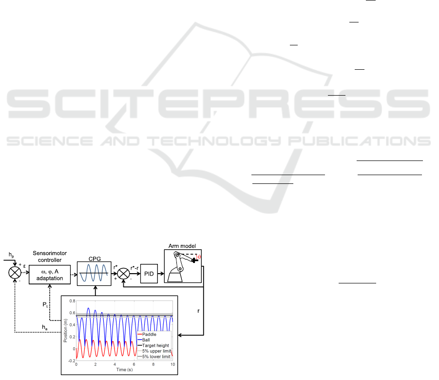
2.3 Bio-inspired Controllers
In the next sections, the study of the different bio-
inspired controllers is achieved by analyzing the fol-
lowing discrete-time representations:
• Map with amplitude and frequency control (Sec-
tion 3.1)
• Approximated map with amplitude and frequency
control (Section 4)
• Map with amplitude, period and phase control
(Section 5)
These representations model the discrete dynam-
ics of the task controlled by the human CPG, that
is viewed as a generator of sinusoidal trajectories.
The additional dynamics introduced by the agent’s
arm mechanical system are supposed to be accurately
canceled by low-level tracking controllers, such as a
PID controller in Figure 2. The arm dynamics are
thus not considered in the present paper. All the pre-
sented results have been achieved for g = 9.81m/s
2
and h
p
= 0.55m.
Figure 2: Block diagram of the ball bouncing closed-loop.
3 HUMAN-LIKE BOUNCING
MAP
In this section, the Poincar
´
e map with amplitude and
frequency control is derived and its stability analyzed.
3.1 Map Definition and Equilibrium
Points
In this case, the Poincar
´
e map of (4) holds, but the am-
plitude A
k
varies according to (5b). The ball apex is
given by h
a
k
= V
2
k
/(2g) + A
k
sin(φ
k
). The paddle fre-
quency being controlled by ω
k+1
= πg/V
k
, the bounc-
ing map is:
A
k+1
= A
k
+ λ(h
p
− A
k
sin(φ
k
) −
V
2
k
2g
) (6a)
V
k+1
= −αV
k
+ (1 +α)A
k+1
πg
V
k
cos(φ
k+1
)
+ α
V
k
π
(φ
k+1
− φ
k
) (6b)
A
k+1
sin(φ
k+1
) −A
k
sin(φ
k
) −
V
2
k
πg
(φ
k+1
− φ
k
)
+
V
2
k
2π
2
g
(φ
k+1
− φ
k
)
2
= 0 (6c)
For
¯
φ solution of (6c), such that φ
k+1
=
¯
φ + 2π,
the equilibrium point of (6) is given by considering
V
k+1
= V
k
=
¯
V and A
k+1
= A
k
=
¯
A:
¯
A =
h
p
(1+α)πcos(
¯
φ)
2(1−α)
+ sin(
¯
φ)
,
¯
V =
s
(1 +α)
¯
Aπgcos(
¯
φ)
(1 −α)
(7)
It can be noted that no equilibrium point exists for
¯
φ in ]π/2,3π/2[ as
¯
V would be undefined. In addition,
only the realistic (positive) values of the paddle am-
plitude are considered. For
¯
A to be positive,
¯
φ must
be inside the interval ]φ
lim
,π/2[ with the limit phase
value φ
lim
given by:
φ
lim
= arctan
−(1 + α)π
2(1 − α)
(8)
Figure 3 presents a comparison between the tra-
jectory variables A
k
and V
k
as functions of the im-
pact number k, predicted by the bouncing map (6) or
resulting from the numerical simulations of the con-
tinuous ball and paddle trajectories. The figure illus-
trates the good matching between the predicted and
simulated variables and underlines the interest of an-
alyzing the task stability properties by focusing on the
presented Poincar
´
e section corresponding to the ball-
paddle impact.
ICINCO 2017 - 14th International Conference on Informatics in Control, Automation and Robotics
488
3.2 Linear Stability Analysis
The Jacobian matrix of (6) is given by:
J =
∂A
k+1
∂A
k
∂A
k+1
∂V
k
∂A
k+1
∂φ
k
∂V
k+1
∂A
k
∂V
k+1
∂V
k
∂V
k+1
∂φ
k
∂φ
k+1
∂A
k
∂φ
k+1
∂V
k
∂φ
k+1
∂φ
k
(9)
with the partial derivatives given by:
∂A
k+1
∂A
k
= 1 − λsin(φ
k
),
∂A
k+1
∂V
k
= −
λV
k
g
∂A
k+1
∂φ
k
= −λA
k
cos(φ
k
)
∂V
k+1
∂A
k
= (1 + α)
πg
V
k
(cos(φ
k+1
)
∂A
k+1
∂A
k
− A
k+1
sin(φ
k+1
∂φ
k+1
∂A
k
)) +
αV
k
φ
k
∂φ
k+1
∂A
k
∂V
k+1
∂V
k
= (1 + α)πg(
∂A
k+1
∂V
k
V
k
− A
k+1
V
2
k
cos(φ
k+1
)
−
A
k+1
V
k
∂φ
k+1
∂V
k
sin(φ
k+1
)) − α
+
α
π
(φ
k+1
− φ
k
+V
k
∂φ
k+1
∂V
k
)
∂V
k+1
∂φ
k
= (1 + α)
πg
V
k
(
∂A
k+1
∂φ
k
cos(φ
k+1
)
− A
k+1
∂φ
k+1
∂φ
k
sin(φ
k+1
))
+
αV
k
π
(
∂φ
k+1
∂φ
k
− 1)
∂φ
k+1
∂A
k
= −
∂F/∂A
k
∂F/∂φ
k+1
,
∂φ
k+1
∂V
k
= −
∂F/∂V
k
∂F/∂φ
k+1
∂φ
k+1
∂φ
k
= −
∂F/∂φ
k
∂F/∂φ
k+1
(10)
with F being the left-hand side of the implicit Equa-
tion (6c).
The Jacobian matrix J in (9) is evaluated at the
equilibrium point (7) and its eigenvalues are denoted
ev
1
, ev
2
, ev
3
. It can be shown that ev
1
and ev
2
are two
hyperbolic eigenvalues. ev
2
is stable (|ev
2
| < 1), for
any value of α and λ whereas ev
1
has a stability that
essentially depends on the value of λ. These results
are demonstrated in the next Section when compared
to the ones of the approximated map. On the con-
trary, ev
3
was shown to be independent of the values
of α and λ, and always equal to unity. ev
3
is thus
non-hyperbolic but also non-defective. It is thus pos-
sible to conclude that the linearized system is Lya-
punov stable, but nothing can be directly deduced
for the nonlinear Poincar
´
e map stability (Stuart and
Humphries, 1998). The bouncing map (6) is thus sin-
gular. Indeed, in addition to the fact that ev
3
= 1, it
Impact number
2 4 6 8 10 12 14
Paddle amplitude (m)
0.12
0.13
0.14
0.15
0.16
Simulator ?
0
=-0.31 (rad)
Bouncing map ?
0
=-0.31
Simulator ?
0
=-0.11
Bouncing map ?
0
=-0.11
Simulator ?
0
=0.08
Bouncing map ?
0
=0.08
a)
Impact number
2 4 6 8 10 12 14
Ball post-impact velocity (m/s
-1
)
3.2
3.3
3.4
3.5
3.6
Simulator ?
0
=-0.31 (rad)
Bouncing map ?
0
=-0.31
Simulator ?
0
=-0.11
Bouncing map ?
0
=-0.11
Simulator ?
0
=0.08
Bouncing map ?
0
=0.08
b)
Figure 3: Comparison of the bouncing map predictions and
simulation of a) the amplitudes series and b) the ball post-
impact velocity series. Three values of the the initial impact
phase φ
0
(λ = 0.09) are considered.
can be seen that (6) is identically zero for any steady-
state value of
¯
φ. Numerical simulations suggest that
the continuum of equilibrium points defined by rela-
tions (7), with
¯
φ a free variable in ]φ
lim
,π/2[, is sta-
ble. During simulated trials, the value of
¯
φ was also
shown to vary only slightly from its initial value φ
0
,
which lead us to the approximation presented in the
next Section.
4 THE HIGH BOUNCE MAP
APPROXIMATION
The implicit equation of the bouncing map presented
in the previous section is approximated by an explicit
equation in the present section to simplify the stabil-
ity analysis. The validity of the approximation is con-
firmed by comparison with numerical simulations.
4.1 Approximated Bouncing Map and
Equilibrium Points
In order to provide an explicit form to the time map
(4b), the high bounce approximation is commonly
considered. This approximation supposes that the
paddle displacement amplitude is small compared to
the ball apex (Holmes, 1982), (Vincent and Mees,
2000), (Vincent, 1995). In that case, one has V
−
k+1
=
Dynamic Stability of Repeated Agent-Environment Interactions During the Hybrid Ball-bouncing Task
489

−V
k
. As V
−
k+1
= V
k
− g(t
k+1
− t
k
), the time map of
the high bounce approximation is given by t
k+1
−t
k
≈
2V
k
/g. As a consequence, according to (2), the ball
velocity after impact is given by: V
k+1
= αV
k
+ (1 +
α)V
r
k+1
. The high bounce map (HBM) with frequency
and amplitude control is:
V
k+1
= αV
k
+ (1 + α)A
k+1
ω
k+1
cos(φ
k+1
) (11a)
A
k+1
= A
k
+ λ(h
p
− A
k
sin(φ
k
) −V
2
k
/(2g)) (11b)
and
¯
φ is given by the trivial phase map φ
k+1
= φ
k
+2π
and thus
¯
φ = φ
0
(mod2π).
This approximated bouncing map is compared to
numerical simulations of the complete system contin-
uous dynamics for validation. Let V
0
, A
0
and φ
0
be
the initial state values of (11). For different values
of λ and specific initial and environmental conditions,
Figure 4a) compares the transient evolution of the ball
apex h
a
of the simulated solution of (6) to the one
calculated with the high bounce map (11). It can be
seen that the dynamics of the task are well described
by the proposed approximated map, and that chang-
ing the value of λ does not modify the equilibrium
but changes the task transient dynamics. Figure 4b)
shows that when V
0
changes, the equilibrium point is
not modified and it can be seen that the simulations
indeed converge towards
¯
V calculated thanks to rela-
tion (7). Figure 4c) shows that, as expected, when φ
0
is modified, the equilibrium point is modified and is
well predicted by (7).
By simulation, it was observed than φ varied by
less than 10% of its initial value φ
0
during trials, for
values of φ
0
inside [−π/4, 2π/5]. As a consequence,
the high bounce approximation is acceptable for this
interval. The reader should nevertheless keep in mind
that outside this interval, the high bounce map mod-
eling accuracy decreases even if the whole phase in-
terval ]φ
lim
,π/2[ is considered for the stability anal-
ysis presented bellow. This accuracy limitation does
not prevent the method to provide information about
the human behavior as it was observed experimen-
tally that almost all the impact phases of humans were
in [−π/4,2π/5] (Sternad et al., 2001), (Siegler et al.,
2010).
4.2 Linear Stability Analysis
The Jacobian matrix of (11) is given by:
J =
∂A
k+1
∂A
k
∂A
k+1
∂V
k
∂V
k+1
∂A
k
∂V
k+1
∂V
k
!
(12)
with the partial derivatives given by:
∂A
k+1
∂A
k
= 1 − λsin(φ
k
) (13a)
∂A
k+1
∂V
k
= −
λV
k
g
(13b)
∂V
k+1
∂A
k
=
−πgcos(φ
k+1
)(α + 1)(λsin(φ
k
) − 1)
V
k
(13c)
∂V
k+1
∂V
k
= α − πλcos(φ
k+1
)(α + 1)
−
πgcos(φ
k+1
)(α + 1)(A
k
+ λ(h
p
− h
a
k
))
V
2
k
(13d)
J evaluated at the equilibrium point is thus equal to
(with
¯
φ = φ
0
(mod2π)):
J
∗
=
1−λsin(
¯
φ) −
λ
¯
V
g
−πgcos(
¯
φ)(α+1)(λsin(
¯
φ)−1)
¯
V
2α−πλcos(
¯
φ)(α+1)−1
!
(14)
The eigenvalues of J
∗
have a complex expression
that will not be presented in the present paper. The
influence of α,λ and φ
0
on the system linear stability
is analyzed in the following paragraphs.
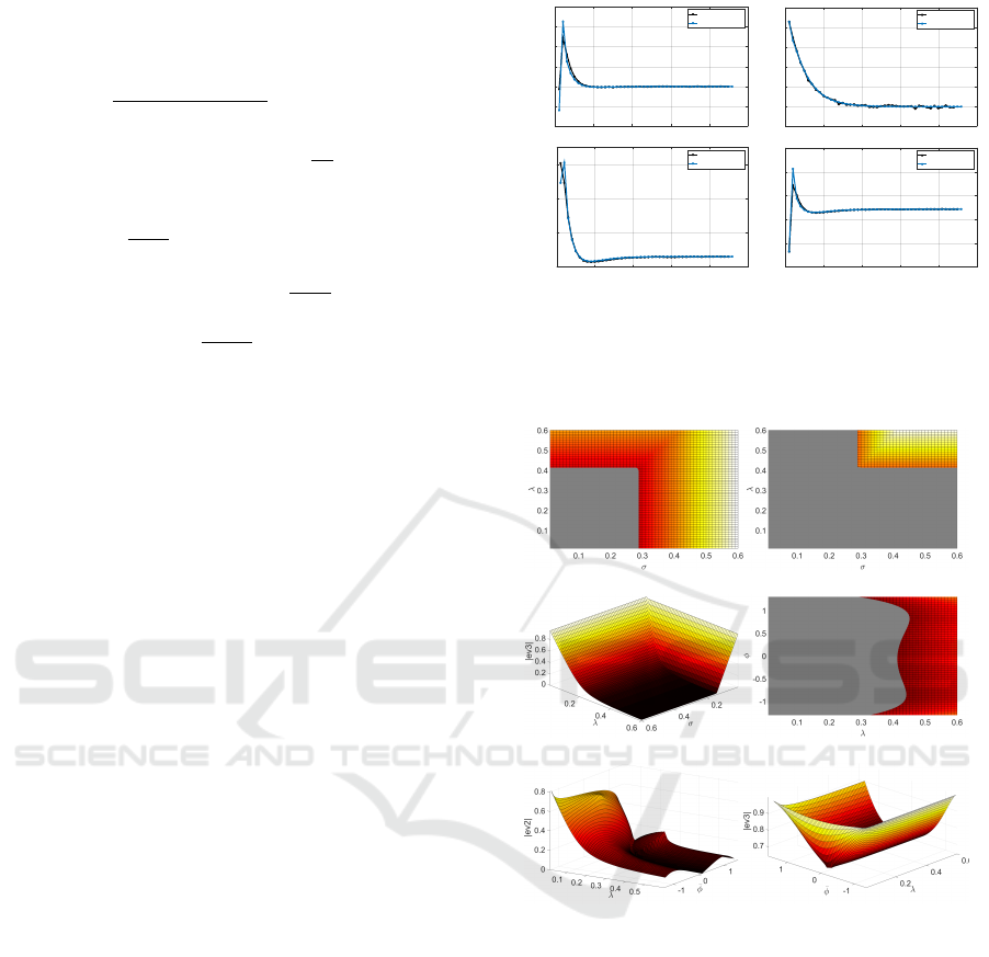
4.3 Influence of the High Bounce
Approximation on the Stability
Figure 5 represents the influence of λ and
¯
φ on the two
hyperbolic eigenvalues |ev
1
| and |ev
2
|, for α = 0.48
and
¯
φ in ]φ
lim
,π/2[. As mentioned in Section 3.2,
it can be seen that ev
2
is always stable whereas the
stability of ev
1
depends on the value of λ, that has
to be lower than 0.4 for the system to be asymp-
totically stable for any value of
¯
φ. For appropriate
value of λ, ev
1
and ev
2
are thus hyperbolic stable.
For
¯
φ inside the considered interval ]φ
lim
,π/2[ and
away from the extreme values, the stability predic-
tion of the approximated map, with the limit λ value
equal to 0.4, matches the one of the high bounce map.
This validity interval is acceptable considering that
the human bouncing phase is localized in the interval
[−π/4,2π/5] as recalled in Section 4.1.
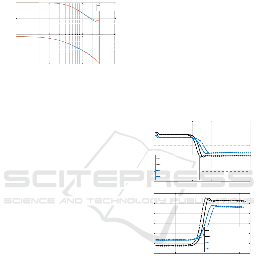
Finally, even if stable, the bouncing maps (6) and
(11) have transient dynamics that depends greatly on
the value of α, as shown in Figure 6. Indeed, the
equilibrium node shape is a stable hyperbolic node
for α around 0.1 (Figure 6a) and b), real eigenval-
ues and −1 < ev
1
< ev
2
< 1), a stable one-tangent
node for α around 0.55 (−1 < ev
1
= ev
2
< 1) and
a stable spiral (elliptic point) for α around 0.9 (Fig-
ure 6c) and d), ev
1
and ev
2
complex, conjugate and
|
ev
1
|
=
|
ev
2
|
< 1). The influence of α on the eigenval-
ues real parts and imaginary parts of the approximated
and non-approximated maps is evidenced in Figure
7. It can be noted that this influence is very similar
ICINCO 2017 - 14th International Conference on Informatics in Control, Automation and Robotics
490
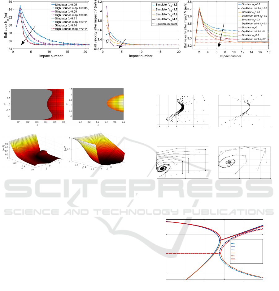
λ↗
a)
V
0
↗
b)
λ↗
c)
Figure 4: Evolution of a) the ball apex for different values of λ (V
0
= 3.2, φ
0
= π/6) b) the ball velocity after impact for
different values of V
0
(λ = 0.09, φ
0
= π/6) and c) the ball velocity after impact for different values of φ
0
(V
0
= 3.2, λ = 0.09).
The three graphs are represented as a function of the impact number. For each simulation, α = 0.48, A
0
= 0.15.
a)|ev
1
|
b)|ev
1
|
c)|ev
2
| d)|ev
2
|
Figure 5: Left column concerns the non-approximated map
and right column the high bounce map. a) and b) represent
|ev
1
|. c) and d) represent |ev
2
|. Eigenvalues are plotted as
a function of
¯
φ and λ. The grey area on Figures a) and b)
corresponds to |ev| < 1 (stable area). The Figures c) and
d) are represented in 3D plots as the second eigenvalue is
always lower than unity.
for the high bounce map and non-approximated map,
confirming the pertinence of the approximation.
As a particular case of the previously presented
Poincar
´
e maps with amplitude and frequency control,
one can notice that if only the period is controlled
while the amplitude remains constant, then the ap-
proximated and non-approximated maps are identi-
cal. They have one trivial eigenvalue equal to 1, cor-
responding to the relation φ
k+1
= φ
k
+ 2π, and one
eigenvalue equal to 2α − 1 that is hyperbolic stable
as α ∈ ]0, 1[. The system is thus linearly ( asymptot-
ically) stable regardless of the environmental condi-
tions.
4.4 Estimation of the Attraction
Domain
For the approximated and non-approximated maps, if
the value of the paddle amplitude A is not forced to be
positive, the domain of initial conditions leading to a
stable bouncing and a convergence towards the equi-
librium point of (7) depends on the values of α, g, λ
Paddle oscillation amplitude A (m)
0.23 0.24 0.25 0.26 0.27 0.28
Ball velocity after impact V (m/s)
2
2.5
3
a)α = 0.1
Paddle oscillation amplitude A (m)
0.2 0.22 0.24 0.26 0.28
Ball velocity after impact V (m/s)
2
2.5
3
3.5
b)α = 0.1
Paddle oscillation amplitude A (m)
0 0.05 0.1 0.15
Ball velocity after impact V (m/s)
2
3
4
5
6
c)α = 0.9
Paddle oscillation amplitude A (m)
0 0.02 0.04 0.06 0.08 0.1
Ball velocity after impact V (m/s)
2
2.5
3
3.5
4
4.5
d)α = 0.9
Figure 6: Left column concerns the non-approximated map
and right column the high bounce map. Nodes shapes a)
and b) for α = 0.1, c) and d) for α = 0.9 and A forced to be
non-negative (λ = 0.09, φ
0
= 0.5,A
0
= 0.15).
,
0.2 0.4 0.6 0.8
Real and imaginary parts of the Jacobian eigenvalues
-0.5
0
0.5
Real(ev1) bouncing map
Imag(ev1) bouncing map
Real(ev2) bouncing map
Imag(ev2) bouncing map
Real(ev1) HBM
Imag(ev1) HBM
Real(ev2) HBM
Imag(ev2) HBM
Figure 7: Real and imaginary parts of the approximated (red
lines) and non-approximated (blue lines) Jacobian eigenval-
ues, as functions of α (λ = 0.09,
¯
φ = 0.5).
and
¯
φ. For a specific equilibrium point defined by
¯
φ,
the attraction domain can be estimated by uniformly
selecting pairs of initial conditions values
{
V
0
, A
0
}
and analyzing the corresponding steady-state behav-
ior (stable or chaotic). This estimation of the stability
domain was achieved for both the approximated and
non-approximated maps, and they were shown to be
the same. As a consequence, Figure 8 only shows the
resulting attraction domain for the non-approximated
Dynamic Stability of Repeated Agent-Environment Interactions During the Hybrid Ball-bouncing Task
491
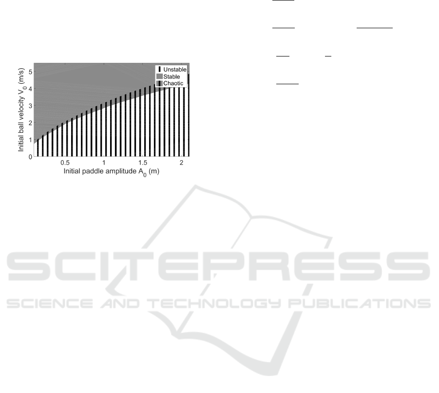
map. The region of the figure with the superimposed
stable and unstable areas is a chaotic region where
small variations of the initial conditions can lead the
system to converge or diverge. On the contrary, when
a saturation is added on the Poincar
´
e maps, forcing A
to stay positive, and for a value of λ lower than 0.4,
the system is stable for any real positive values of V
0
and A
0
.
Figure 8: Attraction domain for α = 0.48, g = 9.81, λ =
0.09, φ
0
= 0.5. 400000 pairs are uniformly selected be-
tween predefined extreme values (V
0
∈ [−5, 5] and A
0
∈
[0,2.2]).
.
4.5 Comparison with a LQR Controller
A parrallel can be drawn between the proposed non-
linear human-like controller and more traditional con-
trol methods. Considering the linearization of the
high bounce map around an equilibrium point. The
human-like controller takes the form of a linear state-
feedback. An equivalent LQR controller formulation
can be found. It is considered that the agent detects
φ
0
at the first impact. For a specific
¯
φ = φ
0
(mod2π),
there is only one equilibrium point given by the re-
lation (7) that cancels the bounce error. It is thus
possible to design a state feedback controller driving
the state (A
k
,V
k
) towards the reference value (
¯
A,
¯
V ).
Here, a LQR controller controls the paddle amplitude
whereas the paddle frequency is controlled to be equal
to the ball frequency as in the previous sections. The
LQR controller is designed based on the linearization
of the map (11). The linear map can be written as:
X
k+1
U
k
=
˜
A
˜
B
0 1
X
k
U
k−1
+
˜
B
1
∆U
k
(15a)
Y
k
=
˜
C
1
˜
C
2
X
k
U
k−1
(15b)
with X
k
= V
k
−
¯
V , U
k
= A
k+1
−
¯
A, Y
k
= h
a
k
− h
p
and :
˜
A =
∂X
k+1
∂X
k
{
¯
A,
¯
V
}
= 2α − 1 (16a)
˜
B =
∂X
k+1
∂U
k−1
{
¯
A,
¯
V
}
= (1 + α)
cos(φ
0
)πg
¯
V
(16b)
˜
C
1
=
∂Y
k
∂X
k
{
¯
A,
¯
V
}
=
¯
V
g
(16c)
˜
C
2
=
∂Y
k
∂U
k−1
{
¯
A,
¯
V
}
= sin(φ
0
) (16d)
Let Z
k
be the state vector
X
k
U
k−1
∈ R
2
. A LQR
controller ∆U
k
= − [K
1
K
2
]Z
k
(∈ R) can be derived
for this linear map by solving a well-known Ric-
cati equation (Kwakernaak and Sivan, 1972). This
controller minimizes the cost function
+∞
∑
k=1
Z
>
k
QZ
k
+
R∆U
2
k
, with Q and R two positive matrices (∈
M
2,2
(R)).
The closed-loop LQR map is thus equal to:
A
k+1
= K
2
¯
A + (1 − K
2
)A
k
− K
1
(V
k
−
¯
V ) (17a)
V
k+1
= αV
k
+ (1 + α)A
k+1
πgcos(φ
0
)/V
k
(17b)
It can be noticed that the human-like con-
troller linearized around the equilibrium point has
a form similar to the LQR one: ∆U
k
= −λY
k
=
−λ
˜
C
1
˜
C
2
Z
k
.
The matrices Q and R were chosen so that the
eigenvalues of (17) were equal to the one of the
human-like bouncing map (11) (the eigenvalues of the
later being equal to the ones of the linearized bounc-
ing map (15) controlled by the linearized human-
like controller). For λ = 0.09, φ
0
= 0.5,α = 0.48,
the eigenvalues of (6) are
{
−0.0625,0.6121
}
. For
Q = 0.013
˜
C
1
˜
C
2
T
˜
C
1
˜
C
2
and R = 1, the eigen-
values of (15) are
{
−0.0396,0.6096
}
. It can be seen
on the Bode plot of Figure 9 that the dynamics of the
closed-loop systems controlled by the linear human-
like controller and by the LQR controller are very
similar. However, the LQR controller has the disad-
vantages of supposing that the relation between the
equilibrium point and the initial conditions is known a
priori, as it integrates
¯
A and
¯
V in (17a). The eigenval-
ues and the stability properties thus depend on h
p
and
g. In the other hand, the system (17) was converging
for any real positive values of A
0
and V
0
tested. The
attraction domain of the LQR controller is thus larger
than the one of the human-like controller presented in
Figure 8, for the environmental conditions tested.
ICINCO 2017 - 14th International Conference on Informatics in Control, Automation and Robotics
492
Magnitude (dB)
-10
0
LQR
Human-like
10
-2
10
-1
10
0
10
1
Phase (deg)
-180
-90
0
Frequency (rad/s)
Figure 9: Bode plot of the closed-loop bouncing map for
the LQR and the human-like controller.
5 POINCAR
´
E MAP WITH PHASE
CONTROL
In the stability analysis of Section 4.3, the system was
shown to be stable provided that λ is lower than an
identified limit value. This stable bouncing was en-
sured even for positive paddle impact acceleration, i.e.
outside the passive stability regime identified in (Di-
jkstra et al., 2004), (Schaal et al., 1996). However,
as recalled in Section 2.2, participants were shown
to generally hit the ball with an impact phase inside
the passive stability regime, corresponding to a spe-
cific interval of negative paddle accelerations at im-
pact. The question of whether this behavior is the
result of a conscious strategy, with the impact phase
actively controlled to converge towards this regime,
or the result of an unconscious process resulting from
the task passive dynamics themselves is investigated
in the following paragraphs.
5.1 The Passive Hypothesis
In the present paragraph it is suggested that partici-
pants tuned into the passive stability regime, not in-
tentionally, but actually because the paddle frequency
control may not be always active. It can indeed be
observed that if the frequency adaptation is switched
off during a steady-state trial and that a very small
perturbation is introduced on the paddle frequency,
then either the ball impact phase converges toward
the passive stability regime because of the passive dy-
namics of the task, or diverges. In the divergence
case, the agent would switch the frequency adapta-
tion back on to stabilize the bouncing. To evidence
the passive convergence case, both numerical simula-
tions of the task continuous dynamics and computa-
tions of the Poincar
´
e map (6) predictions were per-
formed. During the first 15 impacts of a trial, the
paddle period was adapted to equal the ball period
on a cycle basis. Then the active frequency con-
trol is switched off and a small perturbation is added
on the paddle frequency of frequency adaptation law
ω
k+1
= πg/V
k
+ randn/500. The convergence to-
wards the passive stability regime for both the sim-
ulation and the Poincar
´
e map is shown in Figure 10
for two different values of φ
0
. This Figure shows that
during these two trials, after the active frequency con-
trol was switched off, the bouncing was indeed driven
by the passive dynamics of the task towards the pas-
sive stability regime. The Poincar
´
e map (6) accu-
rately predicts this passive convergence observed with
the continuous-time simulations. It can be noted that
the convergence or divergence of the bouncing, after
the active control is switched off, can be predicted
by looking at the attraction domain of the open-loop
Poincar
´
e map presented in (Dijkstra et al., 2004).
Impact number
0 10 20 30 40 50
Paddle impact acceleration (m.s
-2
)
-15
-10
-5
0
5
10
Simulator ?
0
=-:/10
Bouncing map ?
0
=-:/10
Simulator ?
0
=-:/10
Bouncing map ?
0
=-:/10
a)
Impact number
0 10 20 30 40
Impact phase (deg)
-30
-20
-10
0
10
20
30
Simulator ?
0
=-:/10
Bouncing map ?
0
=-:/10
Simulator ?
0
=-:/8
Bouncing map ?
0
=-:/8
b)
Figure 10: Examples of trials converging towards a new
limit cycle inside the passive stability regime when the fre-
quency control is switched off a) Paddle acceleration at im-
pact. The red dashed lines represent the upper and lower
values of the passive stability regimes for the mathematical
expression given in (Dijkstra et al., 2004) b) Impact phase
(λ = 0, A
0
= 0.15).
5.2 The Active Control Hypothesis
In this Section, in addition to the active control of
the ball amplitude, the ball-paddle phase at impact is
considered to be controlled through an adaptation of
the paddle frequency control of (5a). The paddle pe-
riod is adapted on a cycle basis so that T
r
(k + 1) =
Dynamic Stability of Repeated Agent-Environment Interactions During the Hybrid Ball-bouncing Task
493
T
b
(k + 1) + σ(φ
k
− φ
∗
), with φ
∗
the objective impact
phase and σ an adaptation coefficient. The Poincar
´
e
map is thus given by (18):
ω
k+1
=
2π
σ(φ
k
− φ
∗
) + 2V
k
/g
(18a)
A
k+1
= A
k
+ λ(h
p
− A
k
sin(φ
k
) −
V
2
k
2g
) (18b)
V
k+1
= −αV
k
+ (1 + α)A
k+1
ω
k+1
cos(φ
k+1
)
+
αg
ω
k+1
(φ
k+1
− φ
k+1
) (18c)
A
k+1
sin(φ
k+1
) = A
k
sin(φ
k
) +
V
k
ω
k+1
(φ
k+1
− φ
k
)
−
g
2ω
2
k+1
(φ
k+1
− φ
k
)
2
(18d)
The comparison of the ball bouncing perfor-
mances predicted by the bouncing map (18) to simu-
lations led to an accurate matching and highlights the
relevance of the task stability analysis focused on the
discrete-time dynamics. An example of such compar-
ison is given in Figure 11.
The Jacobian matrix takes the same form as in
(9), with the same state. The eigenvalues of the Ja-
cobian matrix evaluated at the equilibrium point have
complex expressions that will not be presented in the
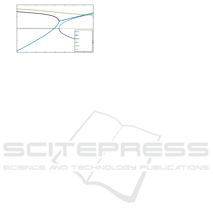
present paper. Figure 12 represents the influence of
λ, σ and
¯
φ = φ
∗
on the Jacobian absolute eigenvalues.
It can be seen that the third eigenvalue, that was non-
hyperbolic in Section 3.2 (|ev
3
| = 1), is now hyper-
bolic and always stable (|ev
3
| < 1) (Figures c) and f)).
The first eigenvalue is stable for σ < 0.3 and λ < 0.4
(Figures b) and e)). For σ < 0.3, the second eigen-
value is stable for any value of λ. To summarize,
the active impact phase control does not provide ad-
ditional stability to the system (the limit value of λ is
the same than the one without active phase control,
according to Figure 12d)), and requires an a priori
knowledge of φ
∗
. However, it is interesting to note
that with active phase control, the Poincar
´
e map is not
singular anymore and the equilibrium point is unique.
It is possible to conclude that the equilibrium point
defined by relations (7) and
¯
φ = φ
∗
is asymptotically
stable without the need for Poincar
´
e map approxima-
tion. The influence of α on the real and imaginary
parts of the three eigenvalues is shown in Figure 13.
6 CONCLUSIONS
The ball-bouncing task has in several past studies
constituted a benchmark to analyze the generation of
rhythmic movement in humans. Previous experimen-
tal studies proposed hypotheses about amplitude, pe-
riod and phase adaptation laws, that were confronted
Impact number
0 10 20 30 40 50
Ball apex (m)
0.45
0.5
0.55
0.6
0.65
0.7
0.75
Simulator
Bouncing map
a)
Impact number
0 10 20 30 40 50
Impact phase (deg)
-5
0
5
10
15
20
25
Simulator
Bouncing map
b)
Impact number
0 10 20 30 40 50
Paddle amplitude (m)
0.12
0.13
0.14
0.15
Simulator
Bouncing map
c)
Impact number
0 10 20 30 40 50
Ball post-impact velocity (m.s
-1
)
2.8
3
3.2
3.4
3.6
3.8
Simulator
Bouncing map
d)
Figure 11: Example of comparison of the bouncing perfor-
mances simulated and predicted by the Poincar
´
e map with
a) the apex series, b) the phase series, c) the paddle ampli-
tude series, d) the ball velocity after impact series. Here
λ = 0.09, σ = 0.05, φ
∗
= 0.5.
a)|ev
1
| b)|ev
2
|
c)|ev
3
| d)|ev
1
|
e)|ev
2
| f)|ev
3
|
Figure 12: For different values of σ (α = 0.48, λ = 0.09),
a) represents |ev
1
|, b) |ev
2
|, c) |ev
3
|. For different values of
λ (α = 0.48, σ = 0.05), d) represents |ev
1
|, e) |ev
2
|, f) |ev
3
|.
The gray area on Figures a), b), d) corresponds to |ev| < 1
(stable area). Figures c), e) and f) are represented in 3D
plots because the corresponding eigenvalue is always lower
than unity.
to an asymptotic stability analysis in the present study.
Conclusions about their verisimilitude were derived
and their stability consequences were identified.
The human adaptation strategies of the paddle os-
cillation amplitude and period were shown to effi-
ciently stabilize the bouncing map. The equilibrium
points stability was assessed for values of the discrete-
time integrator coefficient λ lower than a limit value
0.4. The nonlinear human-like controller was shown
to be equivalent to a LQR controller around an equi-
librium point, while requiring no a priori knowledge
ICINCO 2017 - 14th International Conference on Informatics in Control, Automation and Robotics
494
,
0.1 0.2 0.3 0.4 0.5 0.6 0.7 0.8
Jacobian eigenvalues
-1
-0.5
0
0.5
1
Real(ev1)
Imag(ev1)
Real(ev2)
Imag(ev2)
Real(ev3)
Imag(ev3)
Figure 13: Real and imaginary parts of the Jacobian eigen-
values, as a function of α, for the bouncing map with active
phase control (λ = 0.09, σ = 0.05, φ
∗
= 0.5).
about the equilibrium point.
Notwithstanding the stability of the task with ac-
tive amplitude and frequency control assessed in the
present paper, participants are shown to hit the ball
in the passive stability regime (Sternad et al., 2001).
The present papers analyzed two alternatives justifi-
cations: the impact phase is either actively controlled
by participants or unconsciously driven by the passive
dynamics of the task. The study showed that the ac-
tive impact phase control does not increase stability
that would otherwise justify a voluntary control. It
is also shown that if at one moment of the trial the
active frequency control is switched off, then the pad-
dle acceleration is driven by the passive dynamics of
the task and goes back to the passive stability regime.
This second hypothesis thus seems more likely to ex-
plain the observed human behavior.
Finally, the efficient prediction of the human con-
trol strategies stability was achieved without simulat-
ing the whole continuous and discrete dynamics of the
system. For robotic applications, with the objective
of identifying the control paradigm that gives humans
such a dexterity to achieve tasks in interaction with
the environment, the present study proposes a method
to discard unnecessary control hypotheses while fa-
cilitating the controller adaptation coefficients setting.
The method can be extended to other tasks involving
repeated robot-environment interactions and reduces
the computation time of the robustness tests by avoid-
ing simulation of the task continuous dynamics.
ACKNOWLEDGEMENTS
This work was supported by the Foundation for Sci-
entific Cooperation (FSC) Paris-Saclay Campus.
REFERENCES
Avrin, G., Makarov, M., Rodriguez-Ayerbe, P., and Siegler,
I. A. (2016). Particle swarm optimization of Mat-
suoka’s oscillator parameters in human-like control of
rhythmic movements. In Proc. IEEE American Con-
trol Conf.
Buehler, M., Koditschek, D. E., and Kindlmann, P. (1990).
A simple juggling robot: Theory and experimentation.
In Exp. Rob. I, pages 35–73. Springer.
Choudhary, S. K. (2016). Lqr based optimal control of
chaotic dynamical systems. Int. J. of Modelling and
Simulation, 35(3-4):104–112.
de Rugy, A., Wei, K., M
¨
uller, H., and Sternad, D. (2003).
Actively tracking passive stability in a ball bouncing
task. Brain Research, 982(1):64 – 78.
Dijkstra, T., Katsumata, H., de Rugy, A., and Sternad, D.
(2004). The dialogue between data and model: pas-
sive stability and relaxation behav. in a ball-bouncing
task. Nonlinear Studies, pages 11:319–344.
Holmes, P. J. (1982). The dynamics of repeated impacts
with a sinusoidally vibrating table. J. of Sound and
Vibration, 84(2):173–189.
Kulchenko, P. and Todorov, E. (2011). First-exit model pre-
dictive control of fast discontinuous dynamics: Appli-
cation to ball bouncing. In Robotics and Auto. (ICRA),
2011 IEEE Int. Conf. on, pages 2144–2151. IEEE.
Kwakernaak, H. and Sivan, R. (1972). Linear optimal con-
trol Systems, volume 1. Wiley-interscience New York.
Morice, A., Siegler, I. A., Bardy, B., and Warren, W. (2007).
Action-perception patterns in virtual ball bouncing:
combating syst. latency and tracking functional va-
lidity. Experimental Brain Research, pages 181:249–
265.
Ronsse, R. and Sepulchre, R. (2006). Feedback control
of impact dynamics: the bouncing ball revisited. In
Proc. of the 45th IEEE Conf. on Decision and Con-
trol, pages 4807–4812. IEEE.
Schaal, S., Sternad, D., and Atkeson, C. G. (1996). One-
handed juggling: A dynamical approach to a rhythmic
movement task. J. of Mot. Behav., 28(2):165–183.
Siegler, I. A., Bardy, B. G., and Warren, W. H. (2010). Pas-
sive vs. active control of rhythmic ball bouncing: the
role of visual information. J. of Exp. Psychol. Hum.
Percept. and Perform., 36(3):729–50.
Siegler, I. A., Bazile, C., and Warren, W. (2013). Mixed
control for perception and action: timing and error
correction in rhythmic ball-bouncing. Exp. Brain Res.,
226(4):603–615.
Sternad, D., Duarte, M., Katsumata, H., and Schaal, S.
(2001). Bouncing a ball: tuning into dynamic stabil-
ity. J. of Exp. Psychol. Hum. Percept. and Perform.,
27(5):1163.
Stuart, A. and Humphries, A. R. (1998). Dynamical sys-
tems and numerical analysis, volume 2. Cambridge
University Press.
Tufillaro, N., Mello, T., Choi, Y., and Albano, A. (1986).
Period doubling boundaries of a bouncing ball. J. de
Physique, 47(9):1477–1482.
Dynamic Stability of Repeated Agent-Environment Interactions During the Hybrid Ball-bouncing Task
495

Vincent, T. L. (1995). Controlling a ball to bounce at a fixed
height. In American Control Conf., Proc. of the 1995,
volume 1, pages 842–846. IEEE.
Vincent, T. L. and Mees, A. I. (2000). Controlling a bounc-
ing ball. Int. J. of Bifurcation and Chaos, 10(03):579–
592.
Williamson, M. (1999). Designing rhythmic motions using
neural oscillators. In Proc. IEEE/RSJ Int. Conf. on
Intelligent Robots and Syst.s (IROS), volume 1, pages
494–500 vol.1.
Yu, J., Tan, M., Chen, J., and Zhang, J. (2014). A sur-
vey on CPG-inspired control models and syst. imple-
mentation. IEEE Trans. Neural Netw. Learn. Syst.,
25(3):441–456.
ICINCO 2017 - 14th International Conference on Informatics in Control, Automation and Robotics
496
