Second-order Taylor Stability Analysis of Isolated Kinematic
Singularities of Closed-chain Mechanisms
Adri
´
an Peidr
´
o,
´
Oscar Reinoso, Arturo Gil, Jos
´
e Mar
´
ıa Mar
´
ın, Luis Pay
´
a and Yerai Berenguer
Systems Engineering and Automation Department, Miguel Hern
´
andez University, 03202, Elche, Spain
Keywords:
Closed-chain Mechanism, Isolated Singularity, Taylor Expansion, Stability.
Abstract:
When the geometric design of a closed-chain mechanism is non-generic, the singularity locus of the mecha-
nism may exhibit isolated points. It is well known that these isolated points are unstable since they disappear
or generate/reveal cusps when the geometric design of the mechanism slightly deviates from a non-generic
design, possibly affecting the ability of the mechanism to reconfigure without crossing undesirable singulari-
ties. This paper presents a method based on second-order Taylor expansions to determine how these isolated
singularities transform when perturbing the different geometric parameters of a non-generic mechanism. The
method consists in approximating the singularity locus by a conic section near the isolated singularity, and
classifying the resulting conic in terms of the perturbations of the different geometric parameters. Two non-
generic closed-chain mechanisms are used to illustrate the presented method: an orthogonal 3R serial arm
with specified position for its tip, and the planar Stewart parallel platform.
1 INTRODUCTION
This paper presents a method based on second-order
Taylor expansions to study the stability of isolated
kinematic singularities in closed-chain mechanisms.
Isolated singularities are a type of higher-order kine-
matic singularities of closed-chain mechanisms which
have an important impact on the kinematics of these
mechanisms. Their importance is due to the fact that
these isolated singularities are related to the ability of
the mechanism to reconfigure itself to attain a larger
operational space without crossing undesirable singu-
lar configurations, at which the kinetostatic properties
of the mechanism suffer important changes.
The problem studied in this paper is formulated
next, based on the formulation introduced in (Thomas
and Wenger, 2011). First, consider a closed-chain
mechanism with 2 degrees of freedom (DOF). This is
the usual practice when studying the singularities of
closed-chain mechanisms, since this allows us to vi-
sualize and analyze the singularity locus of the mech-
anism in a plane, which is simpler and more intu-
itive. If the mechanism to be studied has more than
two degrees of freedom, then one only needs to lock
all the degrees of freedom except for two and/or an-
alyze only an independent 2-DOF sub-mechanism of
the complete mechanism (Thomas and Wenger, 2011;
Caro et al., 2012).
Consider two kinematic variables x = [x
1
,x
2
]
T
of
this 2-DOF closed-chain mechanism as inputs, and
other two kinematic variables y = [y
1
,y
2
]
T
as outputs.
These inputs and outputs can be variables defining
the relative position and/or orientation between two
links of interest of the considered mechanism. The
choice of input and output variables depends on the
type of problem to analyze (e.g., the forward or in-
verse kinematic problem of the mechanism). Assume
that, due to the geometric and assembly constraints of
the mechanism, x and y are related by the following
system of two scalar input-output equations:
f
1
(x,y) = 0 AND f
2
(x,y) = 0 (1)
where f
1
and f
2
are constraint functions. In this paper,
we define the Finite Displacement Problem (FDP) as
the problem consisting in solving the outputs y from
Eq. (1) for given inputs x. In general, the FDP has
many different solutions for the same inputs x, i.e.:
FDP: x → Solve y from Eq. (1) → {y
1
,...,y
m
}
where m is the number of different solutions. As in
(Thomas and Wenger, 2011), in this paper we will re-
fer to the different solutions of the FDP (for a given
input x) as assembly modes.
This paper focuses on the singularities of the FDP,
which are the configurations at which det(J) = 0,
where J = { j
pq
} is the 2 × 2 Jacobian matrix of
Peidró, A., Reinoso, Ó., Gil, A., Marín, J., Payá, L. and Berenguer, Y.
Second-order Taylor Stability Analysis of Isolated Kinematic Singularities of Closed-chain Mechanisms.
DOI: 10.5220/0006428503510358
In Proceedings of the 14th International Conference on Informatics in Control, Automation and Robotics (ICINCO 2017) - Volume 2, pages 351-358
ISBN: Not Available
Copyright © 2017 by SCITEPRESS – Science and Technology Publications, Lda. All rights reserved
351

derivatives of { f
1
, f
2
} with respect to the outputs:
j
pq
=
∂ f
p
∂y
q
(p,q ∈ {1,2}). The condition det(J) = 0
defines the singularity locus of the mechanism. The
singularity locus can be represented both in the input
plane (x
1
-x
2
) and in the output plane (y
1
-y
2
), obtain-
ing the singularity curves in these planes. When ap-
proaching these singularity curves in the input plane,
at least two different assembly modes y
a
and y
b
(a 6=
b) coalesce. When the mechanism crosses a singular
configuration, it suffers a loss of dexterity or control
(depending on the nature of the chosen inputs).
In this paper, we are interested in analyzing the
stability of isolated points of the singularity curves
(isolated singularities). When the geometric design
of a closed-chain mechanism satisfies some very spe-
cific conditions (which depend on the particular topol-
ogy of the mechanism), it is said that the geometry of
the mechanism is non-generic and, in that case, the
singularity curves of the mechanism exhibit isolated
points [or other higher-order singularities (Thomas
and Wenger, 2011)]. These isolated points are unsta-
ble, since if the geometry of the mechanism slightly
deviates from the non-generic design (e.g., due to
finite precision in the manufacturing of the mecha-
nism, which impedes building it with an exact non-
generic geometry), these isolated points disappear or
transform into closed curves with cusps (Thomas and
Wenger, 2011; Coste et al., 2016; Coste et al., 2013).
As it is well known, when describing closed tra-
jectories that enclose these cusps in the input plane,
the mechanism can change its assembly mode without
crossing singularities (Zein et al., 2008; Husty et al.,
2014; DallaLibera and Ishiguro, 2014; Peidr
´
o et al.,
2015; Husty, 2009). This is beneficial to enlarge the
range of operation of the mechanism without signif-
icantly affecting its kinetostatic properties, i.e., with-
out suffering losses of dexterity or control.
Perturbing the geometry of a non-generic mech-
anism can importantly alter its kinematic properties.
For example, if the perturbation of the non-generic
geometry of the mechanism transforms an isolated
singularity into a cusped closed curve, then these
cusps will allow the mechanism to change its assem-
bly mode without crossing singularities. If, on the
contrary, the perturbation destroys the isolated point,
then the mechanism will lose such ability to recon-
figure its assembly mode. Therefore, it is impor-
tant to know how the isolated singularities will trans-
form when the geometry of a non-generic closed-
chain mechanism is perturbed.
This paper presents a method to determine how
the isolated singularities of closed-chain mechanisms
transform when their non-generic geometry is slightly
perturbed. To this end (Section 2), the singularity lo-
cus of the mechanism is approximated near the iso-
lated singularity by its second-order Taylor expan-
sion, which is equivalent to approximating the sin-
gularity locus by a conic section. Then, the stabil-
ity analysis of the isolated singularity reduces to clas-
sifying that conic in terms of the perturbations of
the different geometric parameters of the mechanism.
The presented method is illustrated with two different
closed-chain mechanisms in Sections 3 and 4. Finally,
Section 5 presents the conclusions and future work.
2 STABILITY ANALYSIS
THROUGH SECOND-ORDER
TAYLOR EXPANSION
This section presents a method to study the stability
of isolated kinematic singularities based on a second-
order Taylor expansion. Assume that the singularity
locus in the output plane (y
1
-y
2
) is defined by the fol-
lowing equation:
S(y,g) = 0 (2)
where S(y,g) = det(J). For a given geometry g =
[g
1
,...,g
d
]
T
of the mechanism, the previous equation
defines a set of singularity curves in the y
1
-y
2
plane.
The concrete shape of these curves depends on the ge-
ometry g. Assume that, for a given non-generic geom-
etry g
0
, the singularity curves exhibit an isolated point
at y
0
. Next, S will be approximated by its second-
order Taylor expansion about (y
0
,g
0
):
S(y,g) ≈ S(y
0
,g
0
) +

∂S
∂y
(y
0
,g
0
)

∆y+
+

∂S
∂g
(y
0
,g
0
)

∆g+

∆y
T
,∆g
T

H(y
0
,g
0
)
2

∆y
∆g

(3)
where H is the (symmetric) Hessian matrix of S with
respect to y and g, ∆y = y − y
0
and ∆g = g − g
0
. Note
that S(y
0
,g
0
) = 0 because the point y
0
belongs to the
singularity curves corresponding to the geometry g
0
.
Moreover, since y
0
is an isolated point (thus, a critical
or special point) of these curves, then:
∂S
∂y
(y
0
,g
0
) = [0,0] (4)
which justifies the need for a second-order expansion
[otherwise, the following Eq. (5) would not define a
curve in the output plane]. Substituting (3) into Eq.
(2) yields the equation defining the singularity locus
near the isolated singular point y
0
and near g
0
:
S
g
∆g +

∆y
T
,∆g
T

H(y
0
,g
0
)
2

∆y
∆g

= 0 (5)
ICINCO 2017 - 14th International Conference on Informatics in Control, Automation and Robotics
352

Table 1: DH parameters of the robot shown in Figure 1.
DH parameter → θ d α a
0 → 1 φ
1
0 π/2 d
2
1 → 2 φ
2
−r
2
−π/2 d
3
2 → 3 φ
3
r
3
0 d
4
where S
g
=
∂S
∂g
(y
0
,g
0
). Next, the Hessian H is parti-
tioned as follows:
H =

H
11
H
12
H
T
12
H
22

(6)
where the sizes of H
11
, H
12
and H
22
are 2 × 2, 2 × d
and d × d, respectively. Using this partition of H, Eq.
(5) can be rewritten as follows:

∆y
T
,1


H
11
/2 K
K
T
u

| {z }
C

∆y
1

= 0 (7)
where:
K =
H
12
∆g
2
and u =

∆g
T
H
22
2
+ S
g

∆g (8)
Equation (7) defines a conic in the output plane y
1
-y
2
.
The type of conic defined depends on the coefficient
matrix C (Srinivasan, 2003). Note that C depends on
the perturbation ∆g from the non-generic geometry
g
0
. Thus, to study how the perturbations in the ge-
ometry of the robot affect the stability of the isolated
singularity y
0
, we only need to study and classify the
type of conic defined by C in terms of ∆g.
In the next sections, we will apply this method
to study the stability of isolated singularities in two
closed-chain mechanisms.
3 EXAMPLE 1: ORTHOGONAL
3R SERIAL ARM
This section analyzes the stability of isolated kine-
matic singularities in the orthogonal 3R serial robot
studied in (Thomas and Wenger, 2011). This serial
robot, shown in Figure 1, has three revolute joints ar-
ranged in such a way that consecutive revolute axes
are orthogonal. In this robot, the three joint angles φ
1
,
φ
2
and φ
3
(which are the rotations about the axes z
0
,
z
1
and z
2
of Figure 1, respectively) are used to control
the position p = [p
x
, p
y
, p
z
]
T
of the tip.
The DH parameters of this robot are shown in Ta-
ble 1, where g = [d
2
,d
3
,d
4
,r
2
,r
3
]
T
are the geometric
parameters. Multiplying the corresponding DH ma-
trices yields the position of the tip in terms of φ
i
:
p
x
= c
1
(c
2
(d
4
c
3
+ d
3
) − r
3
s
2
+ d
2
) − s
1
(d
4
s
3
+ r
2
)
(9)
z
2
z
2
x
2
r
3
d
4
x
1
r
2
d
3
x
z
3
Tip (p
x
, p
y
, p
z
)
x
0
y
0
z
0
x
3
z
1
d
2
y
0
Figure 1: Orthogonal 3R serial robot studied in (Thomas
and Wenger, 2011).
p
y
= s
1
(c
2
(d
4
c
3
+ d
3
) − r
3
s
2
+ d
2
) + c
1
(d
4
s
3
+ r
2
)
(10)
p
z
= r
3
c
2
+ s
2
(d
4
c
3
+ d
3
) (11)
where s
i
= sinφ
i
and c
i
= cosφ
i
(i ∈ {1,2,3}). The po-
sition of the tip can also be given in cylindrical coor-
dinates (φ,ρ, p
z
) (Thomas and Wenger, 2011), where
ρ =
q
p
2
x
+ p
2
y
(12)
is the radial coordinate, φ is the polar angle and p
z
is
the height or axial coordinate. Since ρ and p
z
only
depend on the joint angles φ
2
and φ
3
, we can focus
only on the sub-arm composed of these two joints,
and consider that this 2-DOF serial sub-arm is used to
control the radial and axial coordinates of the tip of
the robot (Thomas and Wenger, 2011).
Although this 2-DOF sub-arm is a serial robot
(i.e., with open architecture), specifying the cylindri-
cal coordinates (ρ, p
z
) of its tip transforms it into a
2-DOF closed-loop mechanism in which the inputs
are the specified radial and axial coordinates of the
tip (x = [ρ, p
z
]
T
) and the outputs are the last two joint
angles (y = [φ
2
,φ
3
]
T
). Thus, the Finite Displacement
Problem studied in this section coincides with the in-
verse kinematics of this 2-DOF serial sub-arm.
The input-output equation [Eq. (1)] of this mech-
anism is composed of Eqs. (11) and (12), from which
the constraint functions f
1
and f
2
are identified:
f
1
= −ρ
2
+ c
2
2
(d4
2
c
2
3
+ 2d
3
d
4
c
3
+ d
2
3
)
− c
2
(s
2
(2d
4
r
3
c
3
+ 2d
3
r
3
) − 2d
2
d
4
c
3
− 2d
2
d
3
)
+ r
2
3
s
2
2
− 2d
2
r
3
s
2
+ d
2
4
s
2
3
+ 2d
4
r
2
s
3
+ d
2
2
+ r
2
2
(13)
f
2
= r
3
c
2
+ s
2
(d
4
c
3
+ d
3
) − p
z
(14)
According to Eq. (2), the singularity locus of this
mechanism in the output plane is defined by:
S(y,g) =
∂ f
1
∂φ
2
∂ f
2
∂φ
3
−
∂ f
1
∂φ
3
∂ f
2
∂φ
2
= 0 (15)
Second-order Taylor Stability Analysis of Isolated Kinematic Singularities of Closed-chain Mechanisms
353

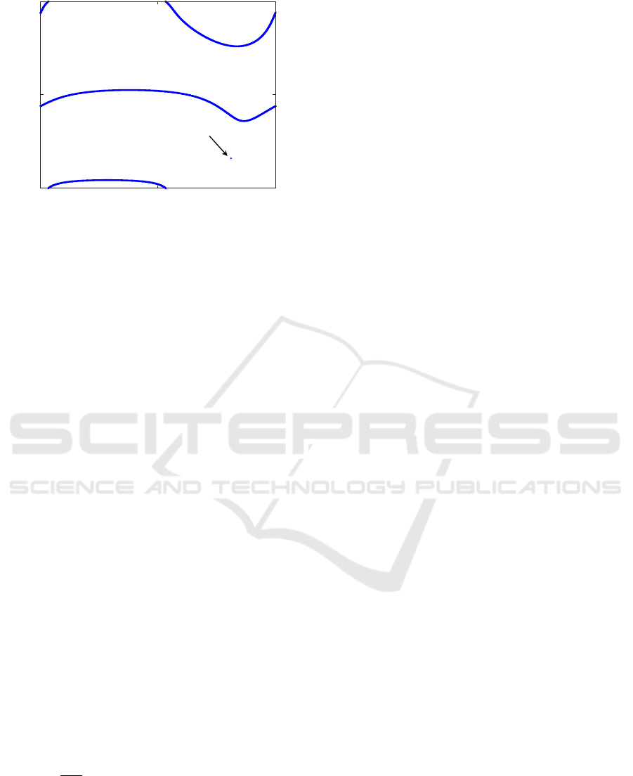
y
0
-3.14
3.14
0
ϕ
3
3.14
-3.14
0
ϕ
2
Figure 2: Singularity locus of a non-generic orthogonal 3R
serial robot in the φ
2
-φ
3
plane.
S only depends on the output variables y = [φ
2
,φ
3
]
T
and on the geometric parameters g (the inputs disap-
pear due to the partial derivatives). The resulting ex-
pression of S(y,g) is not shown here due to its length.
The concrete shape of the singularity curves de-
fined by S(y,g) = 0 will depend on the value of the
geometric parameters g. Next, we will analyze one
of the non-generic geometries studied in (Thomas
and Wenger, 2011), defined by the following values:
g
0
= [1,0.5,0.3327820876,0.2,0.8]
T
. For this geom-
etry, the singularity curves exhibit an isolated point
y
0
= [1.953146918,−2.13618956]
T
rad (see Figure
2). As it is well known (Thomas and Wenger, 2011),
this isolated point is a higher-order unstable singu-
larity [called lips when represented in the ρ-p
z
plane
using Eqs. (12) and (11)], for if the geometry of the
robot slightly deviates from the non-generic geometry
g
0
, then the isolated point y
0
transforms into a loop or
even disappears, possibly altering the kinematic prop-
erties of the mechanism. Applying the analysis pre-
sented in Section 2 will allow us to determine how
y
0
transforms depending on how the geometry of the
mechanism is perturbed away from g
0
.
Next, consider that all the geomet-
ric parameters suffer a small perturbation
∆g = [∆d
2
,∆d
3
,∆d
4
,∆r
2
,∆r
3
]
T
from the non-generic
geometry g
0
indicated in the previous paragraph.
Substituting y
0
and g
0
into Eq. (7) yields the equation
of a conic curve that approximates the perturbed
singularity locus in the output plane φ
2
-φ
3
, where:
H
11
2
=

−0.0904 0.0273
0.0273 −0.1128

(16)
K =





0 −0.1362
0.09725 0.05913
−0.05211 −0.1376
−1.760 · 10
−10
0.2235
−0.03911 0.1348





T
∆g (17)
u = −0.5616∆d
2
∆d
3
− 0.242∆d
2
∆d
4
− 0.1807∆d
2
+ 0.2096∆d
2
3
− 0.1097∆d
3
∆d
4
− 0.1328∆d
3
∆r
2
+ 0.5209∆d
3
∆r
3
+ 0.0008248∆d
3
+ 0.7776∆d
2
4
− 0.8519∆d
4
∆r
2
+ 0.584∆d
4
∆r
3
+ 0.2589∆d
4
− 0.3303∆r
2
∆r
3
− 0.3069∆r
2
+ 0.1941∆r
3
(18)
The type of conic defined by Eq. (7) depends on H
11
,
K and u (Srinivasan, 2003). First, since det(H
11
) >
0, then the perturbed singularity locus is an ellipse
(either real or imaginary). The type of ellipse defined
by Eq. (7) depends on ω = c
11
det(C), where c
11
is the
first element of the first row of C:
• If ω > 0, then Eq. (7) defines an imaginary ellipse.
• If ω < 0, then Eq. (7) defines a real ellipse.
If ω = 0, then the ellipse degenerates into a single
point. The perturbation ∆g of the geometric parame-
ters will determine the sign of ω and, therefore, will
determine the type of ellipse into which the isolated
point y
0
transforms when the geometry of the robot
slightly deviates from the non-generic geometry g
0
.
3.1 Perturbing One Geometric
Parameter
For simplicity, consider first that only d
4
is perturbed,
i.e., ∆g = [0,0,∆d
4
,0,0]
T
[this is the situation studied
in (Thomas and Wenger, 2011)]. In that case:
ω = −(0.0008835∆d
4
+ 0.0002213)∆d
4
(19)
By plotting Eq. (19) (see Figure 3), we can identify
three cases for small perturbations ∆d
4
:
• If ∆d
4
> 0, then ω < 0 → the singularity locus is
a real ellipse.
• If ∆d
4
< 0, then ω > 0 → the singularity locus is
an imaginary ellipse
• If ∆d
4
= 0, then ω = 0 → the singularity locus is
a (real) ellipse shrunk into a point.
Thus, if d
4
is slightly increased from its non-generic
value (∆d
4
> 0), the isolated point y
0
transforms into
a tiny real ellipse E
r
in the φ
2
-φ
3
plane. As ∆d
4
de-
creases and approaches zero, the size of this real el-
lipse continuously decreases, until it shrinks into the
point y
0
when ∆d
4
= 0 (i.e., the isolated point y
0
re-
mains unaltered since the non-generic geometry of the
mechanism is not altered). If the perturbation is fur-
ther decreased and becomes negative (∆d
4
< 0), then
the point y
0
transforms into an imaginary ellipse, i.e.,
y
0
disappears from the (real) φ
2
-φ
3
plane.
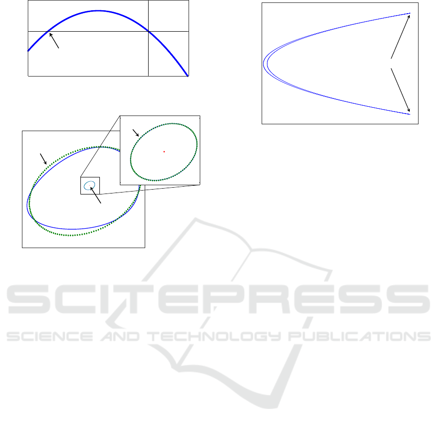
Figure 4a illustrates the transformation of y
0
into
an approximately elliptic loop E
r
for ∆d
4
= 0.0002:
the ellipse defined by Eq. (7) is represented in green
ICINCO 2017 - 14th International Conference on Informatics in Control, Automation and Robotics
354

2·10
-5
-3·10
-5
0
ω
Δd
4
Δd
4
= -0.2504
0 0.1-0.3
Figure 3: Variation of ω with ∆d
4
.
2.211.64
ϕ
2
-2.46
-1.85
ϕ
3
Δd
4
= 0.02
y
0
(b)
y
0
(a)
1.981.92
-2.16
-2.11
E
r
Δd
4
= 0.0002
Figure 4: Transformation of the singularity locus near y
0
into an approximately elliptic loop when perturbing d
4
.
dotted line, whereas the exact singularity locus [de-
fined by Eq. (15)] is represented in blue continuous
line. Note that Eq. (7) approximates the exact sin-
gularity locus very accurately for small perturbations,
but for large perturbations this approximation is not
valid (e.g., see Figure 4b, where ∆d
4
= 0.02).
If the real ellipse E
r
is mapped to the input plane
using Eqs. (11) and (12), then it transforms into a
small closed curve with two cusps (see Figure 5). It is
well known that these cusps allow the mechanism to
reconfigure between different assembly modes with-
out crossing singularities. Thus, the destruction of the
real ellipse corresponds to the destruction of these two
cusps and, therefore, the mechanism loses such ability
to reconfigure without crossing singularities.
The previous results regarding the relationship be-
tween the sign of ∆d
4
and the stability of the iso-
lated point y
0
, obtained by analyzing the sign of ω
in Eq. (19), agree with (Thomas and Wenger, 2011),
where the singularity locus was plotted in the ρ-p
z
plane for different values of d
4
both above and below
the non-generic geometry (d
4
= 0.3327820876).
Note that, according to Figure 3, ω becomes again
negative for ∆d
4
< −0.2504, which means that the
real ellipse E
r
defined by Eq. (7) reappears again
for ∆d
4
< −0.2504. This may erroneously suggest
that the exact singularity locus, defined by Eq. (15),
should also exhibit a small loop due to the reappear-
0.160130.1599
-0.0246
0.025
ρ
p
z
Cusps
Figure 5: Closed curve with two cusps at (ρ ≈
0.16012, p
z
≈ ±0.020653), obtained as the image of the el-
lipse E
r
of Figure 4a in the ρ-p
z
plane.
ance of the ellipse E
r
. However, this is not true be-
cause the perturbation ∆d
4
= −0.2504 is too large for
Eq. (7) to be a valid approximation of the exact sin-
gularity locus. Thus, the analysis of the sign of ω in
Eq. (19) is only valid for sufficiently small values of
|∆d
4
|. It can be checked that, unlike in Figure 4, the
exact singularity locus does not exhibit small (approx-
imately elliptic) loops for ∆d
4
< −0.2504.
3.2 Perturbing Two Geometric
Parameters
Next, consider that both d
4
and r
2
are perturbed
from the non-generic geometry g
0
, i.e.: ∆g =
[0,0,∆d
4
,∆r
2
,0]
T
. In that case, ω equals:
ω = −0.0008835∆d
2
4
+ 0.001289∆d
4
∆r
2
− 0.0002213∆d
4
− 0.0004083∆r
2
2
+ 0.0002625∆r
2
(20)
Figure 6 shows how the sign of ω depends on the per-
turbations ∆d
4
and ∆r
2
. The ∆d
4
-∆r
2
plane is divided
into three regions {R
1
,R
2
,R
3
} by the hyperbola with
branches {h
1
,h
2
}, which is defined by ω = 0. Since
ω < 0 in region R
1
, then Eq. (7) defines a real ellipse
for perturbations falling in that region. This means
that, for perturbations in region R
1
, the isolated point
y
0
deforms into a small (approximately elliptic) loop
in the output plane. This loop transforms into a closed
curve with two cusps when mapped to the input plane
using Eqs. (12) and (11). Figure 7 shows an example
of this, for the following perturbation (which falls in
region R
1
): ∆d
4
= 0.0002, ∆r
2
= −0.0002.
For perturbations falling in R
2
, we have ω > 0 and,
therefore, Eq. (7) defines an imaginary ellipse. This
means that the point y
0
disappears for perturbations
belonging to region R
2
, and the mechanism loses the
Second-order Taylor Stability Analysis of Isolated Kinematic Singularities of Closed-chain Mechanisms
355

21-1-2 0
-2
-1
0
1
2
Δd
4
Δr
2
R
1
(ω < 0)
R
2
(ω > 0)
R
3
(ω > 0)
h
2
h
1
Figure 6: Variation of the sign of ω [Eq. (20)] with the per-
turbations ∆d
4
and ∆r
2
.
φ
2
(a) (b)
ρ
p
z
φ
3
y
0
E
r
0.16053
0.15995
1.991
1.91
-2.175
-2.1
Cusps
Figure 7: (a) An (approximately) elliptic loop E
r
of the sin-
gularity locus of a perturbed orthogonal 3R serial robot. (b)
Image of E
r
in the input plane, which presents two cusps at
(ρ ≈ 0.16047, p
z
≈ ±0.03051).
ability to change between different solutions of the
FDP without crossing singularities.
Finally, it is important to remark again that the
behavior of the exact singularity locus [defined by
Eq. (15)] under large perturbations cannot be pre-
dicted by analyzing the transformations suffered by
the ellipse defined by Eq. (7). For example, according
to Figure 6, the nature of the ellipse defined by Eq. (7)
changes between real and imaginary when crossing
the branch h
2
of the hyperbola ω = 0 (i.e., when both
perturbations ∆d
4
and ∆r
2
are sufficiently negative).
This does not mean that the exact singularity locus of
the mechanism loses an (approximately) elliptic loop
when passing from region R
1
to region R
3
, because
h
2
is crossed for perturbations so large that render the
quadratic approximation of Eq. (7) invalid.
4 EXAMPLE 2: PLANAR
STEWART PLATFORM
In this section, the proposed method will be used to
analyze the stability of the isolated singularities of
Figure 8: General 3RPR planar parallel robot.
the planar Stewart platform. Consider first a general
3RPR planar parallel robot (Figure 8), which is com-
posed of a fixed base AFC and a mobile platform BDE
interconnected by three actuated prismatic limbs (P)
through revolute joints (R). In this robot, three lin-
ear actuators {AB,CD,EF}, with respective lengths
{ρ
1
,ρ
2
,ρ
3
}, are used to control the position and ori-
entation of the triangular platform BDE. The position
of the mobile platform can be parameterized by the
polar coordinates (ρ
3
,θ
3
) of joint E, whereas its ori-
entation can be parameterized by the angle φ.
To apply the method described in Section 2, we
need a 2-DOF closed-chain mechanism. Therefore,
from now on, the prismatic joint of the limb EF will
be locked, and its length ρ
3
will be assumed to be con-
stant. In this way, we will deal with a 2-DOF closed-
chain mechanism with inputs x = [ρ
1
,ρ
2
]
T
and out-
puts y = [θ
3
,φ]
T
. All the remaining parameters indi-
cated in Figure 8 will be considered as geometric de-
sign parameters, i.e., g = [c
2
,c
3
,d
3
,l
1
,l
3
,β,ρ
3
]
T
. For
this mechanism, the input-output equations (1) are ob-
tained by imposing the condition that the lengths of
the limbs AB and CD should be ρ
1
and ρ
2
, respec-
tively. This yields the following constraint functions:
f
1
= −2l
3
ρ
3
c
θ
3
c
φ
+ 2c
3
ρ
3
c
θ
3
− 2l
3
ρ
3
s
θ
3
s
φ
+ 2d
3
ρ
3
s
θ
3
− 2c
3
l
3
c
φ
− 2d
3
l
3
s
φ
+ c
2
3
+ d
2
3
+ l
2
3
+ ρ
2
3
− ρ
2
1
(21)
f
2
= −2l
1
ρ
3
c
β
c
θ
3
c
φ
− 2l
1
ρ
3
c
β
s
θ
3
s
φ
+ 2c
2
l
1
c
β
c
φ
− 2c
3
l
1
c
β
c
φ
− 2d
3
l
1
c
β
s
φ
− 2l
1
ρ
3
s
β
c
θ
3
s
φ
+ 2l
1
ρ
3
s
β
s
θ
3
c
φ
+ 2d
3
l
1
s
β
c
φ
+ 2c
2
l
1
s
β
s
φ
− 2c
3
l
1
s
β
s
φ
− 2c
2
ρ
3
c
θ
3
+ 2c
3
ρ
3
c
θ
3
+ 2d
3
ρ
3
s
θ
3
+ c
2
2
− 2c
2
c
3
+ c
2
3
+ d
2
3
+ l
2
1
+ ρ
2
3
− ρ
2
2
(22)
where s
w
= sin w and c
w
= cos w (w ∈ {β,φ,θ
3
}).
The singularity locus of this mechanism in the output
ICINCO 2017 - 14th International Conference on Informatics in Control, Automation and Robotics
356

plane is defined by the following equation:
S(y,g) =
∂ f
1
∂θ
3
∂ f
2
∂φ
−
∂ f
1
∂φ
∂ f
2
∂θ
3
= 0 (23)
Equation (23) does not depend on the inputs be-
cause they vanish due to the partial derivatives. The
shape of the singularity locus depends on the value
of the geometric design parameters g. In the follow-
ing, we will analyze the singularity locus of the non-
generic geometry analyzed in (Peidr
´
o et al., 2016).
The considered non-generic geometry is defined by
g
0
= [1.5,0.5,0,0.5,0.5,π rad,1]
T
. This geometric
design is non-generic because it implies that the three
joints AFC of the base are perfectly aligned (d
3
= 0),
and also that the three joints BDE of the mobile plat-
form are perfectly aligned (β = π rad). This design of
the 3RPR parallel robot can be considered as a planar
version of the Stewart platform (Haug et al., 1995).
Figure 9 shows the singularity locus in the output
plane corresponding to the considered non-generic
geometry g
0
. This singularity locus exhibits an iso-
lated point at y
0
= [π, 0] rad. Next, we will apply
the analysis of Section 2 to analyze the stability of
this isolated point. Consider that all the geomet-
ric parameters suffer a small deviation from g
0
, i.e.:
∆g = [∆c
2
,∆c
3
,∆d
3
,∆l
1
,∆l
3
,∆β,∆ρ
3
]
T
. Substituting
y
0
and g
0
into Eq. (7), which approximates the singu-
larity locus in the output plane near y
0
, yields:
H
11
2
=

1 −0.25
−0.25 1.5

(24)
K = [1.5∆d
3
− 0.5∆β,−2.5∆d
3
− 0.75∆β]
T
(25)
u = 5∆d
3
∆β − 4∆d
2
3
(26)
Although all the geometric parameters are perturbed,
according to Eqs. (25) and (26), the transformation
of y
0
depends only on the perturbations of d
3
and β,
which are precisely the only two geometric parame-
ters that determine whether g
0
is a generic geometry
or not (since these two parameters determine if the
base and platform joints are respectively aligned). In
the example of Section 3, the transformation of the
isolated singularity depended on the perturbations of
all the geometric parameters [see Eqs. (17) and (18)].
Since det(H
11
) > 0, Eq. (7) defines a real or imag-
inary ellipse, depending on the sign of ω = c
11
det(C):
ω = −1.125(12∆d
2
3
− 5∆d
3
∆β + ∆β
2
) (27)
ω in Eq. (27) is a negative definite quadratic form, i.e.,
ω < 0 ∀(∆d
3
,∆β) 6= (0,0). Therefore, if any of the
two geometric parameters {d
3
,β} deviates from its
non-generic value, then Eq. (7) defines a real ellipse
in the output plane, independently of the direction of
these perturbations. This means that the isolated point
3.14
-3.14
0
6.28
θ
3
ϕ
y
0
Figure 9: Singularity locus of a planar Stewart platform.
y
0
of the exact singularity locus always deforms into
a small loop that can be approximated by an ellipse if
the perturbations are sufficiently small.
If this ellipse is mapped to the input plane, then it
transforms into a deltoid δ, which is a closed curve
with three cusp points (see the example of Figure
10). This deltoid is very important for the kinemat-
ics of the mechanism, since varying the inputs along a
closed trajectory that encloses any of these individual
cusps allows the mechanism to switch between dif-
ferent assembly modes. Encircling the whole deltoid
(i.e., the three cusps simultaneously) also has this ef-
fect (Coste et al., 2016; Peidr
´
o et al., 2016).
In (Peidr
´
o et al., 2016), the following analysis was
presented: departing from the non-generic geometry
g
0
analyzed in this section, the geometric parameters
d
3
and β were numerically perturbed to study how the
mentioned deltoid δ was affected by these perturba-
tions. That analysis showed that the shape and size
of the deltoid δ vary due to these perturbations, and it
degenerates into a point (which is the image of y
0
in
the input plane) when the perturbations tend to zero.
However, no perturbation could be found in (Peidr
´
o
et al., 2016) that destroys the deltoid δ in the same
way that the bicuspidal closed curve of Figure 5 can
be destroyed by rendering the ellipse E
r
(which gen-
erates this bicuspidal curve) imaginary (ω > 0). This
is because a deltoid is a stable singularity obtained
when perturbing a singularity of multiplicity 4, which
is the case of the isolated point y
0
(Coste et al., 2016).
In this aspect, the analysis presented in this section
complements the analysis presented in (Peidr
´
o et al.,
2016) and illustrates the fact that the deltoid δ can-
not be destroyed by any combination of perturbations
from the non-generic geometry g
0
: in the analyzed
3RPR robot, these perturbations always transform the
isolated point y
0
into a real ellipse, and the image of
this real ellipse in the input plane is the deltoid δ.
Second-order Taylor Stability Analysis of Isolated Kinematic Singularities of Closed-chain Mechanisms
357

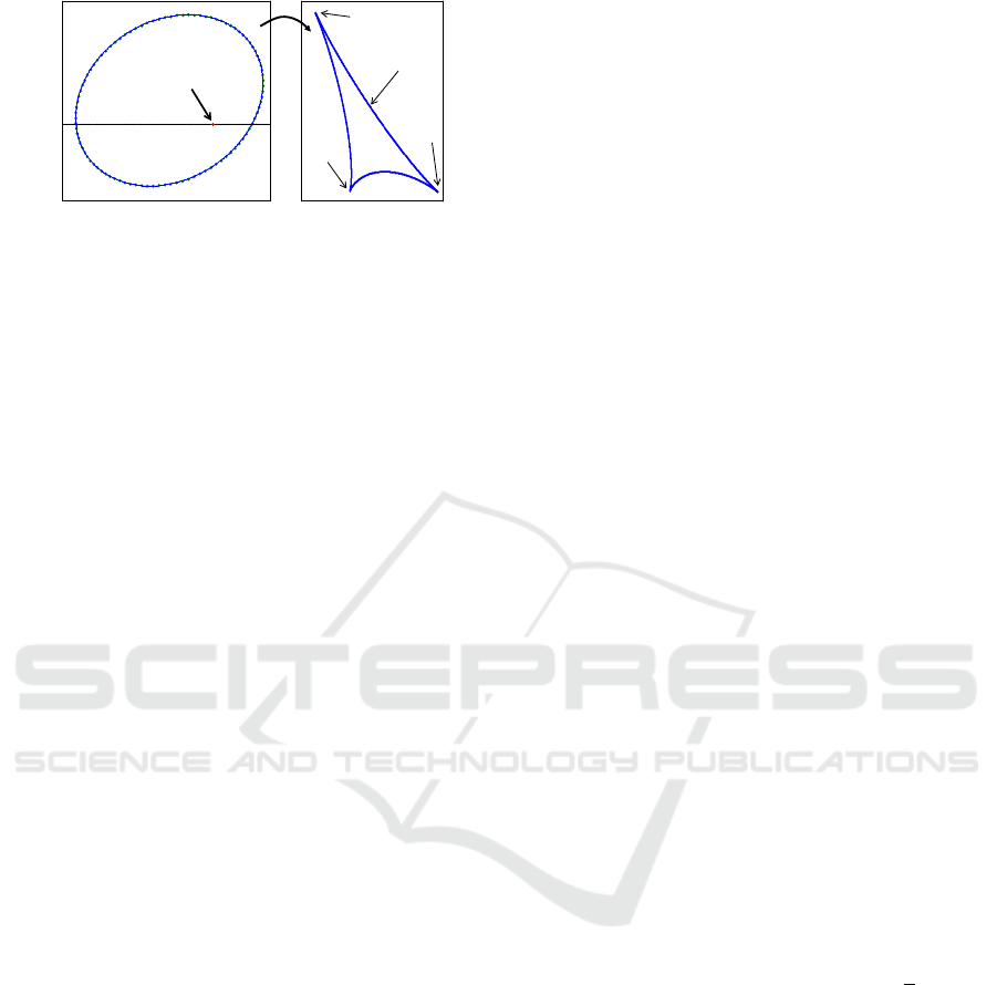
y
0
= [π,0]
θ
3
φ
0
3.08
3.165
-0.028
0.045
(a)
k
1
k
2
k
3
ρ
1
ρ
2
(b)
δ
Figure 10: (a) (Approximately elliptic) singularity locus
near y
0
when the non-generic geometry of a planar Stewart
platform is slightly perturbed (∆d
3
= 0.01, ∆β = −0.01).
(b) The image of this ellipse in the input plane is a deltoid
δ, with cusps: k
1
≈ (0.9995, 1.5014), k
2
≈ (0.9999, 1.4999)
and k
3
≈ (1.0009,1.4999).
5 CONCLUSION
This paper has presented a method to determine
how isolated singularities of closed-chain mecha-
nisms transform when the geometric design param-
eters of the mechanism slightly deviate from a non-
generic design. The method consists in approximat-
ing the singularity locus by a conic section and clas-
sifying it in terms of the perturbations of the different
geometric parameters of the mechanism. The method
has been illustrated with two closed-chain mecha-
nisms whose singularity loci exhibit isolated points.
In the future, we will extend this analysis to other
higher-order singularities besides isolated points, and
to mechanisms with more than 2 DOF. In addition, we
will explore the application of the proposed method in
the robust design of cuspidal parallel robots.
ACKNOWLEDGEMENTS
This work was supported by the Spanish Ministries
of Education (grant number FPU13/00413) and Econ-
omy (project number DPI 2016-78361-R).
REFERENCES
Caro, S., Wenger, P., and Chablat, D. (2012). Non-singular
assembly mode changing trajectories of a 6-DOF par-
allel robot. In The ASME 2012 International Design
Engineering Technical Conferences & Computers and
Information in Engineering Conference, pages 1–10.
Coste, M., Chablat, D., and Wenger, P. (2013). New Trends
in Mechanism and Machine Science: Theory and
Applications in Engineering, chapter Perturbation of
Symmetric 3-RPR Manipulators and Asymptotic Sin-
gularities, pages 23–31. Springer Netherlands, Dor-
drecht.
Coste, M., Wenger, P., and Chablat, D. (2016). Hidden
cusps. In 15th International Symposium on Advances
in Robot Kinematics, pages 1–9.
DallaLibera, F. and Ishiguro, H. (2014). Non-singular tran-
sitions between assembly modes of 2-DOF planar par-
allel manipulators with a passive leg. Mech. Mach.
Theory, 77:182–197.
Haug, E. J., Adkins, F. A., Qiu, C. C., and Yen, J.
(1995). Analysis of barriers to control of manipula-
tors within accessible output sets. In Proceedings of
the 20th ASME Design Engineering Technical Confer-
ence, pages 697–704.
Husty, M. (2009). Non-singular assembly mode change in
3-RPR-parallel manipulators. In Kecskem
´
ethy, A. and
M
¨
uller, A., editors, Computational Kinematics, pages
51–60. Springer Berlin Heidelberg.
Husty, M., Schadlbauer, J., Caro, S., and Wenger, P.
(2014). The 3-RPS manipulator can have non-
singular assembly-mode changes. In Thomas, F. and
P
´
erez Gracia, A., editors, Computational Kinemat-
ics, volume 15 of Mechanisms and Machine Science,
pages 339–348. Springer Netherlands.
Peidr
´
o, A., Gil, A., Mar
´
ın, J. M., Pay
´
a, L., and Reinoso,
´
O. (2016). On the stability of the quadruple solutions
of the forward kinematic problem in analytic paral-
lel robots. Journal of Intelligent & Robotic Systems,
pages 1–16.
Peidr
´
o, A., Reinoso, O., Gil, A., Mar
´
ın, J., and Pay
´
a, L.
(2015). A virtual laboratory to simulate the control of
parallel robots. IFAC-PapersOnLine, 48(29):19–24.
Srinivasan, V. (2003). Theory of Dimensioning: An Intro-
duction to Parameterizing Geometric Models. CRC
Press.
Thomas, F. and Wenger, P. (2011). On the topological char-
acterization of robot singularity loci. a catastrophe-
theoretic approach. In Proceedings of the 2011 IEEE
International Conference on Robotics and Automa-
tion, pages 3940–3945.
Zein, M., Wenger, P., and Chablat, D. (2008). Non-singular
assembly-mode changing motions for 3-RPR parallel
manipulators. Mech. Mach. Theory, 43(4):480–490.
ICINCO 2017 - 14th International Conference on Informatics in Control, Automation and Robotics
358